Data programming and intro to R
Prepare, clean, transform and enrich data in R
Welcome to R!
Put your spreadsheets, SAS and SPSS aside
Hi!
Mail: javalv09@ucm.es.

Javier Álvarez Liébana from Carabanchel (Madrid).
Degree in Mathematics (UCM). PhD in Statistics (UGR).
In charge of data visualization and analysis for the Principality of Asturias (2021-2022) during the COVID pandemic
Member of the Spanish Society of Statistics and OR and the Spanish Royal Mathematical Society.
Currently, Assistant Professor at the Faculty of Statistics of the UCM. Disseminating via Twitter e Instagram
Goals
.png)
Take away the fear of programming → learn to program by programming
Understanding basic R concepts from scratch → learning to abstract ideas and algorithms
Utility of programming → reproducible, transparent and maintainable workflows.
Introduction to analysis and preprocessing of data →
{tidyverse}.Handling advanced data types →
{forcats},{lubridate}and{purrr}packages
Evaluation: intro to R
- Attendance and individual participation (30%)
- Final exam on 10/09/2024, 15:00-16:10 (70%).
- Max grade: to get a grade greater than 9/10 you should get at least 9/10 in the final exam.
Evaluation: data programming
- Attendance and individual participation (10%)
- 2 individual tasks done during the course (20%-25%)
- 1 group task between 4 and 6 people (20%). Deadline: 23/12/2024.
- Final exam with all materials and internet (25%). You are exempt if you get more than 7/10 in the previous tasks.
- Max grade: to get a grade greater than 9/10 you should get at least 9/10 in the individual tasks.
Planning
- Final exam (intro R 70%): 10/09/2024 (15:00 - 16:10).
Individual task I (20%): deadline 03/11/2024
Individual task II (25%): deadline 30/11/2024
Group task (20%): deadline 23/12/2024.
- Final exam (25% if required): TBA
Planning: intro R
Planning: data programming
| LESSON | WEEK | DATES | TOPIC | EX. | WORKBOOK | TASK | |||
|---|---|---|---|---|---|---|---|---|---|
| 1 | S2 | 12 sep | Intro to tidy data | 💻 💻 | 🐣 | ||||
| 2 | S3 | 19 sep | Tidyverse: by rows | 💻 💻 | 🐣 | ||||
| 3 | S4 | 26 sep | Tidyverse: by columns | 💻 💻 | 🐣 🐣 🐣 | ||||
| 4 | S5 | 3 oct | Tidyverse: summary | 💻 | 🐣 🐣 | ||||
| 5 | S6 | 10 oct | Loops | 💻 | 🐣 🐣 | ||||
| 6 | S7 | 17 oct | Functions and joins | 💻 💻 | 🐣 🐣 🐣 | ||||
| 7 | S8 | 24 oct | Import/export | 💻 | 🐣 | ||||
| 8 | S10 | 6 nov | Purrr and forcats packages | 💻 💻 | 🐣 | ||||
| 9 | S11 | 13 nov | Github and SQL connection |
Materials
- Slides: slides made with
Quartoavailable and updated on https://javieralvarezliebana.es/docencia/mucss-data-programming. In the slide menu (bottom left) you have an option to download them in pdf inTools
Material: workbooks and extra materials.
🗃 Data: datasets that will be used, available on https://javieralvarezliebana.es/docencia/mucss-data-programming/material or Google Drive https://drive.google.com/drive/folders/18Ok6Epqcimszqguj_JTTLuSbs5Ot5Srd?usp=sharing
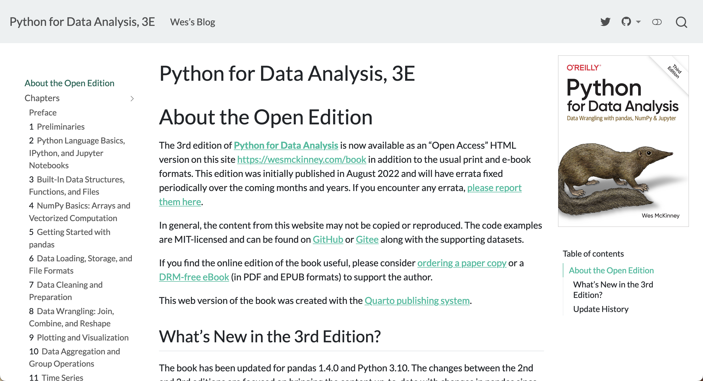
📚 Extra resources: https://r4ds.had.co.nz/, https://cdr-book.github.io/ and https://ivelasq.quarto.pub/intro-to-quarto/.
L1: first steps
Introduction to R and RStudio. Working with projects. First uses of functions and packages. Basic data types
Requirements
For the course, the only requirements will be:
- Internet connection (to download some data and packages).
- Install R: it will be our language. We will download it (for free) from https://cran.r-project.org/
- Install RStudio from https://posit.co/download/rstudio-desktop/

R vs RStudio

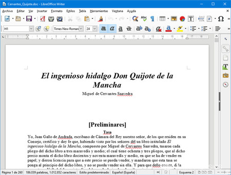
We will program as we write
- We will need a grammar, a language (
R)
- And an environment, such as Word (
RStudio) to write it
Installing R
The R language will be our grammar and spelling (our rules of the game)
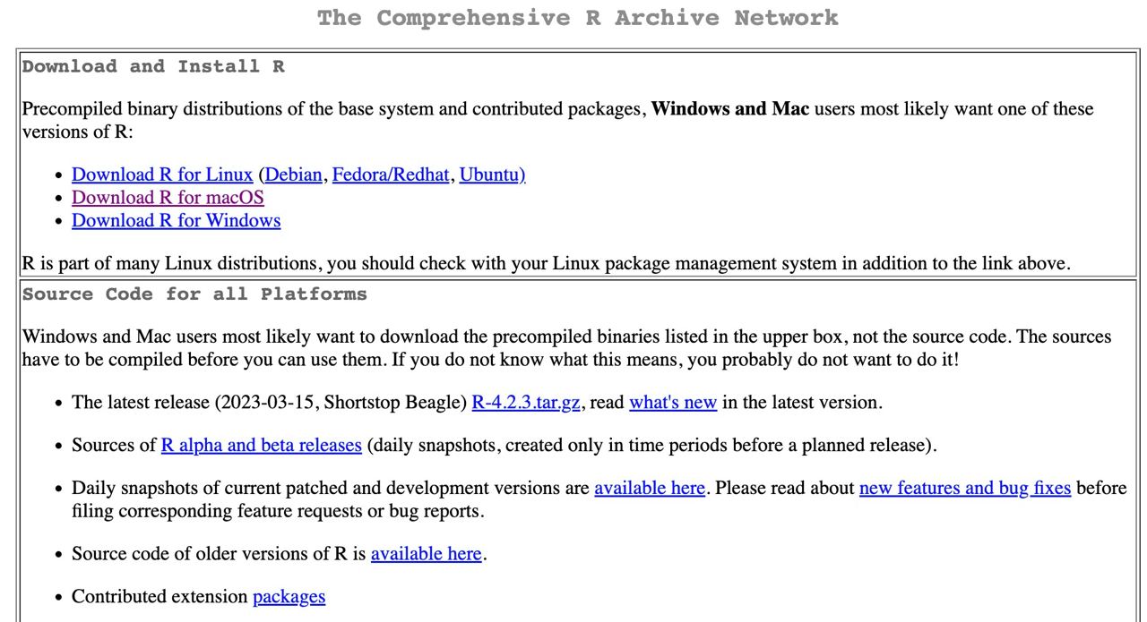
Step 1: go to https://cran.r-project.org/ and select your operating system.
Step 2: for Mac, simply click on the .pkg file, and open it once downloaded. For Windows systems, we need to click on install R for the first time and then on Download R for Windows. Once downloaded, open it like any installation file.
Step 3: open the installation executable.
Cuidado
Whenever you need to download something from CRAN (either R itself or a package), make sure you have an internet connection.
First operation
To check the installation, after opening R, you should see the R GUI (Graphical User Interface) with a white screen similar to this (console).
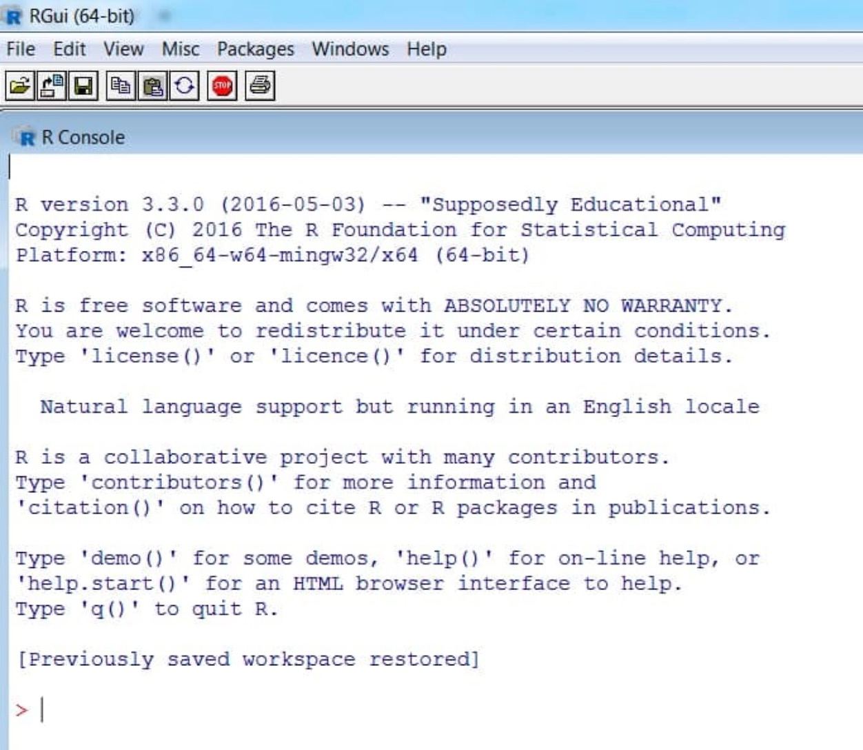
First code: we will assign the value 1 to a variable called a (we will write the code in the console and press “enter”). Then we will do the sum a + b.
First operation
To check the installation, after opening R, you should see the R GUI (Graphical User Interface) with a white screen similar to this (console).

First code: we will assign the value 1 to a variable called a (we will write the code in the console and press “enter”). Then we will do the sum a + b.
First operation
To check the installation, after opening R, you should see the R GUI (Graphical User Interface) with a white screen similar to this (console).

First code: we will assign the value 1 to a variable called a (we will write the code in the console and press “enter”). Then we will do the sum a + b.
Note that…
In the console, a number [1] appears: it’s simply an element counter (like counting rows in Word)
Installing R Studio
RStudio will be the Word we will use to write (what is known as an IDE: Integrated Development Environment).
Step 1: go to the official RStudio website (now called Posit) and select the free download.
Step 2: select the executable that appears according to your operating system.
Step 3: after downloading the executable, open it like any other and let the installation finish.
RStudio Organization
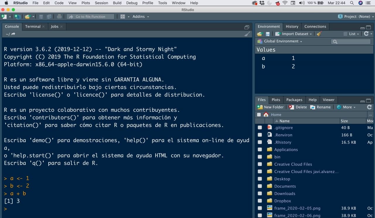
When you open RStudio you will likely have three windows:
- Console: is the name for the large window that takes up most of your screen. Try writing the same code as before (the sum of the variables) in it. The console is where we will execute commands and display results.
RStudio Organization
When you open RStudio you will likely have three windows:
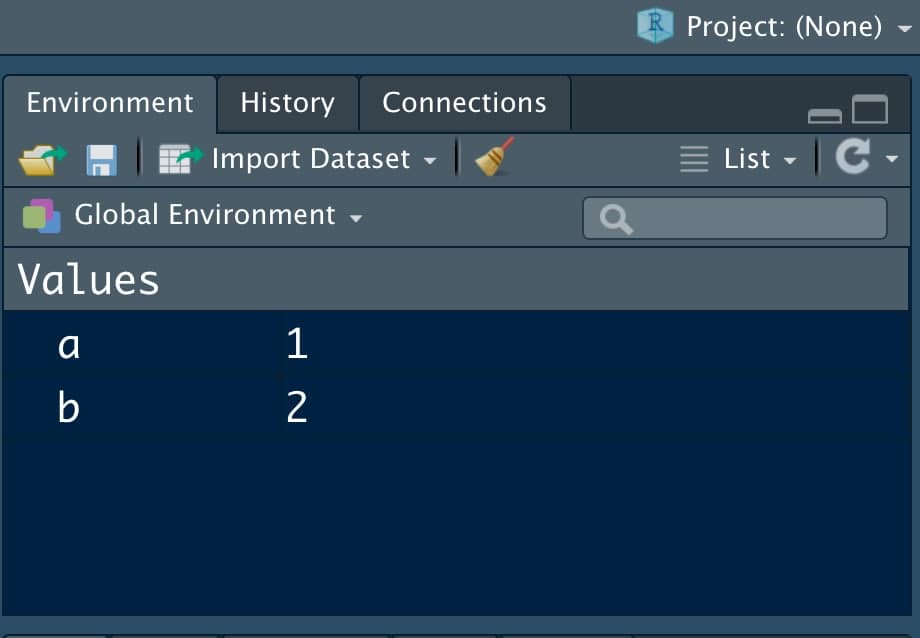
- Environment: the small screen (you can adjust the margins with the mouse to your liking) that we have in the top right corner. It will show us the variables we have defined.
RStudio Organization
When you open RStudio you will likely have three windows:
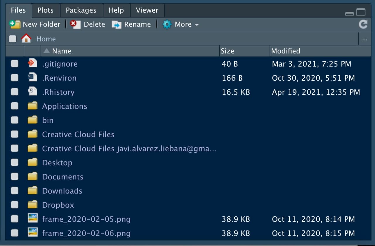
- Multi-purpose panel: the window at the bottom right will be used to look for function help, as well as to visualize plots.
What is R? Why R?

What is R? Why R?
R is the evolution of the work of Bell Laboratories with the S language, which was brought into the open-source world by Ross Ihaka and Robert Gentleman in the 1990s. The version R 1.0.0 was released on February 29, 2000.
What is R? Why R?
R is the statistical language par excellence, created by and for statisticians, with 6 fundamental advantages over Excel, SAS, Stata, or SPSS:
- Programming language: the obvious → replicable analysis
- Free: the philosophy of the
Rcommunity is to share code under copyleft → ethical use of spending and algorithms
- Open-source software: not only is it free, but it also allows free access to others’ code, even to the source code itself → flexibility and transparency (Free and Open Source Software FOSS)
What is R? Why R?
R is the statistical language par excellence, created by and for statisticians, with 6 fundamental advantages over Excel, SAS, Stata, or SPSS:
- Modular language: we have installed the minimum, but there are codes from other people that we can reuse (almost 20,000 packages) → time saving and immediate innovation
- High-level language: facilitates programming (like Python) → lower learning curve
- Community and employability: along with Python, it is the most used language in the field of statistics and data science in research, teaching, companies (Línea Directa, Mapfre, Telefónica, Orange, Apple, Spotify, Netflix, El País, Civio, HP, etc.) and public organizations (ISCIII, CNIC, CNIO, INE, IGN, CIS, CEO, DGT, AEMET, RTVE, etc.)
Why programming?
Automate → it will allow you to automate recurring tasks.
Replicability → you will be able to replicate your analysis in the same way every time.
Flexibility → you will be able to adapt the software to your needs.
Transparency → to be audited by the community.
Fundamental Idea: Packages
One of the key ideas of R is the use of packages: codes that other people have implemented to solve a problem
Fundamental Idea: Packages
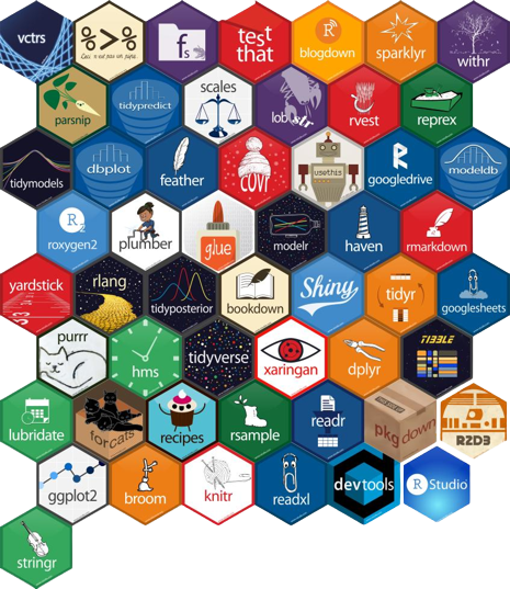
Once installed, there are two ways to use a package (take it off the shelf)
- Whole package: with
library(), using the package name without quotes, we load the whole book into the session
You will be wrong
During your learning, it will be very common for things not to work out on the first try → you will be wrong. It will not only be important to accept it but also to read the error messages to learn from them.
- Error messages: preceded by “Error in…” and will be those failures that prevent execution
Scripts (.R files)
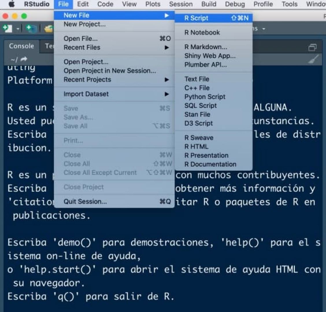
A script will be the document in which we program, our .doc file (here with a .R extension) where we will write the commands. To open our first script, click on the menu in File < New File < R Script.
Be careful
It’s important not to overuse the console: everything you don’t write in a script, when you close, will be lost.
Be careful
R is case-sensitive: it is sensitive to uppercase and lowercase, so x and X represent different variables.
Running the first script
Now we have a fourth window: the window where we will write our codes. How do we run it?
- Write the code to be executed.
- Save the .R file by clicking on
Save current document.
- The code does not execute unless we indicate it. We have three options to run a script:
- Copy and paste into the console.
- Select lines and press
Ctrl+Enter - Enable Source on Save next to save: not only saves but also executes the entire code.
Organizing: projects
Just as we usually work organized by folders on the computer, in RStudio we can do the same to work efficiently by creating projects.
A project will be a “folder” within RStudio, so our root directory will automatically be the project folder itself (allowing us to switch from one project to another using the top right menu).
We can create one in a new folder or in an existing folder.”
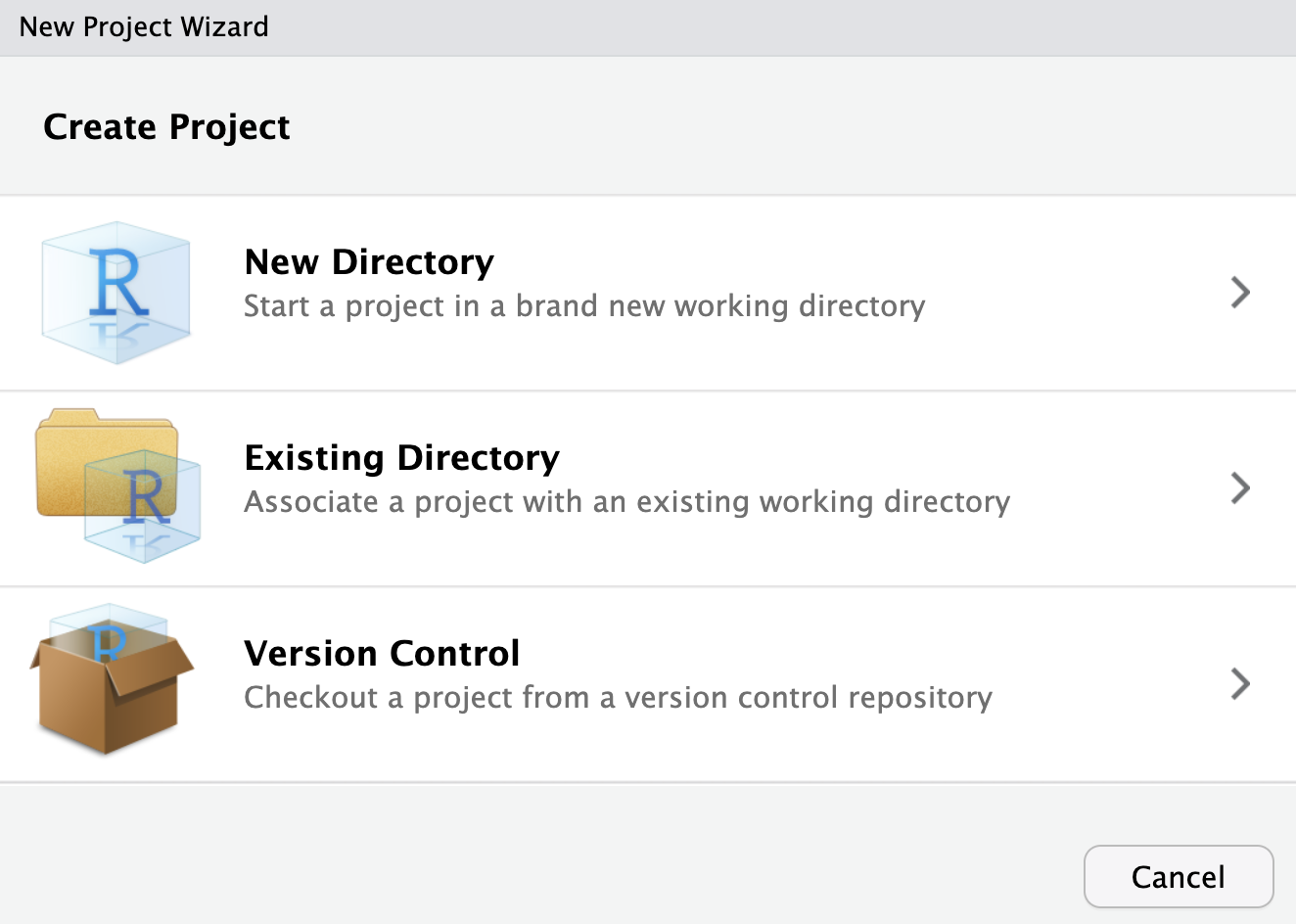
💻 It’s your turn
📝 Create in your computer a folder of the subject and create inside it the RStudio project: it is there where you are going to save everything that we will do along this course, after creating the project you will have an R Project file. Then create in this folder two subfolders: data (this is where you will save the different datasets that we will use) and scripts (this is where you will save the .R files of each class).
📝 Inside the project create a script Exercises-class1.R (inside the scripts folder). Once created, define in it a variable named a and whose value is -1. Execute the code in the (three) ways explained before.
📝 Add below another line to define a variable b with the value 5. Then save the multiplication of both variables. Execute the code as you want.
📝 Modify the code below to define two variables c and d, with values 3 and -1. Then divide the variables and save the result.
📝 Assign to x a positive value and then compute its square root; assign to y a negative number and compute its absolute value using abs().
Note that…
Commands like sqrt(), abs() or max() are what we call functions: lines of code that we have “encapsulated” under a name, and given some input arguments, execute the commands (a sort of shortcut). In the functions the arguments will ALWAYS be enclosed in parentheses
📝 Using the variable x already defined, complete/modify the code below to store in a new variable z the result stored in x minus 5.
📝 Define an x variable and assign it the value -1. Define another y and assign it the value 0. Then perform the operations a) x by y; b) square root of x. What do you get?
From CELL to TABLE
What data type can we have in each cell of a table?
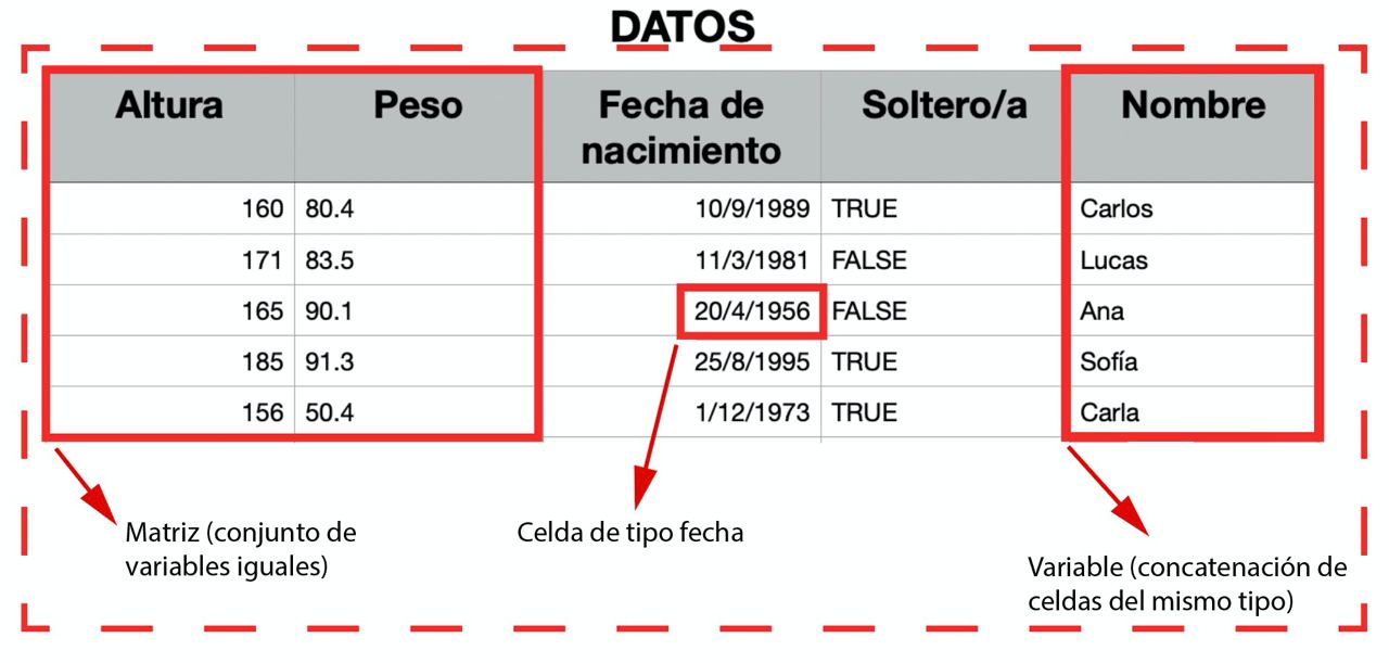
- Cell: an individual piece of data of a specific type.
- Variable: concatenation of values of the same type (vectors in R).
- Matrix: concatenation of variables of the same type and length.
- Table: concatenation of variables of different types but the same length
- List: concatenation of variables of different types and different lengths
But first…best practices
Before we continue, it’s important to know something as soon as possible: starting with programming can be frustrating
Just like when learning a new language, the first obstacle is not so much what to say but how to say it correctly. The same goes for R, so let’s standardize our programming style as much as possible to avoid future errors.
But first…best practices
- Tip 2: program like you write. Just like when writing in Spanish, get used to incorporating spaces and line breaks to avoid making your code hard to read (it’s a good practice, not a requirement, because
Rdoes not process spaces).
- Tip 3: don’t be chaotic, standardize names. Always get used to naming variables consistently. The only requirement is that they must always start with a letter (and without accents). The most recommended form is
snake_case.
But first…best practices
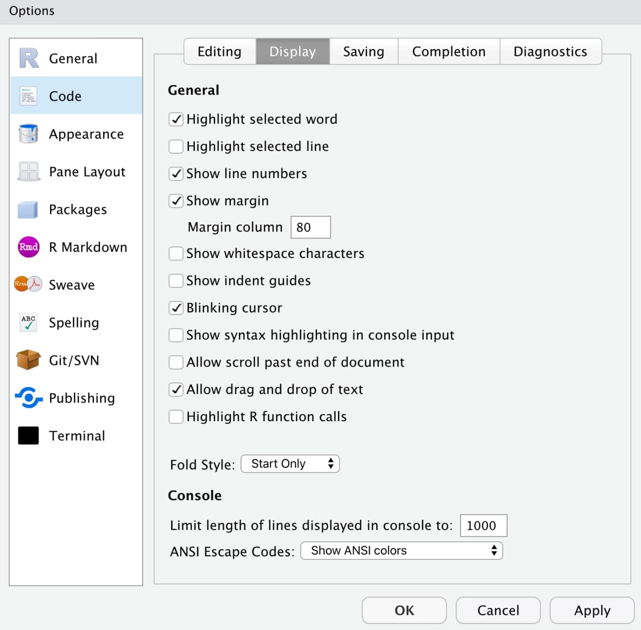
- Tip 4: make reading and writing easier, set limits. In
Tools < Global Options, you can customize some options inRStudio. InCode < Display, you can setShow marginto display an “imaginary” margin (not interacting with the code) to “force” you to make line breaks.
But first…best practices
- Tip 5: the tab key is your best friend. In
RStudio, there’s a wonderful tool: if you type part of a variable or function name and press tab,RStudiowill autocomplete it for you.

But first…best practices
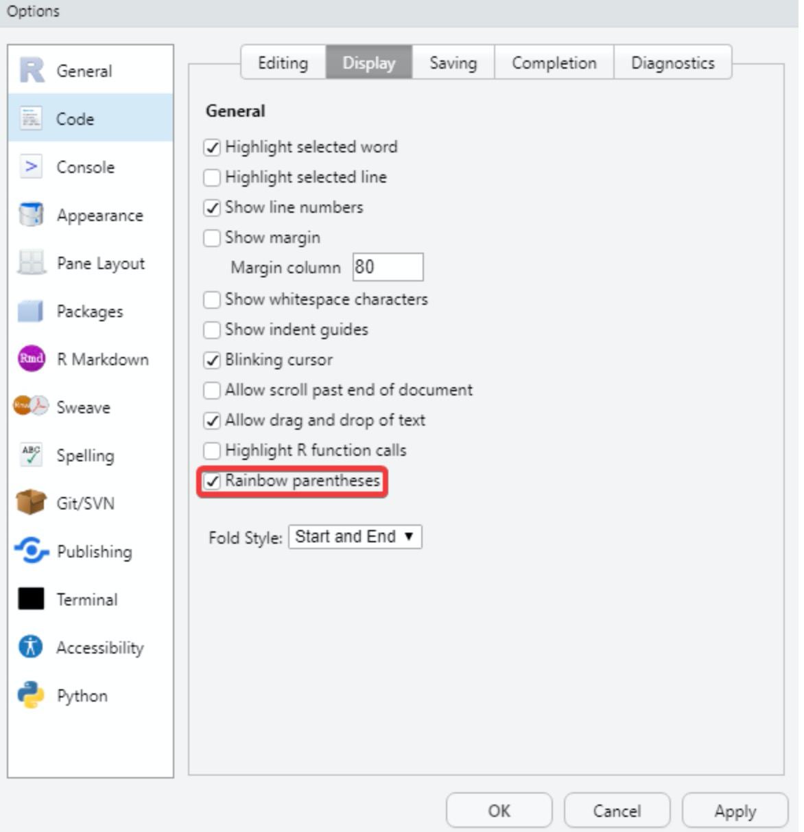
- Tip 6: no single parentheses. Whenever you open a parenthesis, you must close it. To make this task easier, go to
Tools < Global Options < Code < Displayand enable theRainbow parentheses option.
But first…best practices
- Tip 7: pay attention to the left side. You will not only see the line of code you are on but also, in case of a syntax error,
RStudiowill notify you.

- Tip 8: try to always work by projects (for this class, create a script
class1.Rin the project we created before)
See more tips at https://r4ds.had.co.nz/workflow-basics.html#whats-in-a-name
Cells: data types
Are there variables beyond numbers in data science? For example, think about the data you might store about a person:
- The answer to the question “Are you enrolled in the Faculty?” will be what we call a logical variable (
TRUEif enrolled orFALSEotherwise).
- Their date of birth will be precisely that, a date.
Numerical variables
The simplest data (which we’ve already used) will be numeric variables. To find out the data class in R of a variable, we use the class() function.
Numerical variables
The simplest data type (we have already used it) will be the numeric variables. To know the data class in R of a variable we have the function class().
To know its typology (format) variable we have typeof().
[1] "double"[1] "integer"Note that…
In R we have a collection of functions starting with as.x() that serve as conversion functions: a data that was of one type, we convert it to type x.
Numerical variables
In addition to the “common” numbers we will have the plus/minus infinity coded as Inf or -Inf.
Numerical variables
With numeric variables we can perform the arithmetic operations of a calculator: adding (+)…
String variables
Let us imagine that, in addition to the age of a person we want to store his/her name: now the variable will be of type character.
The text strings are a type with which we obviously cannot perform arithmetic operations (other operations such as pasting or locating patterns can be performed).
Reminder
Text variables (character or string) are ** ALWAYS in quotes**: TRUE (logical, binary value) is not the same as "TRUE" (text).
First function: paste
As we have commented R we will call function a piece of encapsulated code under a name, and which depends on some input arguments. Our first function will be paste(): given two strings, it allows us to paste them together.
First function: paste
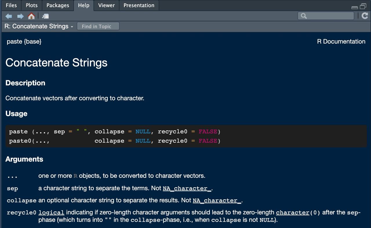
How do I know what arguments does a function need?
By typing ? paste in the console, you will get a help in the multipurpose panel, where you can see in its header what arguments the function already has default arguments assigned to it.
First function: paste
The arguments (and their detail) can also be consulted by tabulating (after a comma).

Functions: default arguments
It is very important to understand the concept of default argument of a function in R: it is a value that the function uses but sometimes we may not see because already has a value assigned.
[1] "Javi Álvarez"[1] "Javi Álvarez"Fíjate que...
The = operator is reserved for assigning arguments within functions. For all other assignments, we will use <-.
First package: glue
A more intuitive way to work with text is to use the {glue} package: the first thing to do is to “buy the book” (if we have never done it before). After that load the package
With the glue() function of that package we can use variables inside strings. For example, “age is … years old”, where the age is stored in a variable.
Logical variables
Another fundamental type will be the logical or binary variables (two values):
TRUE: true stored internally as a 1.FALSE: false stored internally as a 0.
Logical variables
As we will see shortly, logical variables can actually take a third value: NA or missing data, representing not available, and it will be very common to find it within a database.
Logical conditions
Logical values are usually the result of evaluate logical conditions. For example, imagine that we want to check whether a person is named Javi.
With the logical operator == we ask if what we have stored on the left is same as what we have on the right: we ASK
Note that…
It is not the same <- (assignment) as == (we are asking, it is a logical comparison).
Logical conditions
In addition to “equal to” versus “different” comparisons, also order comparisons such as less than <, greater than >, <= or >=. Is the person less than 32 years old?
Date variables
A very special data type: the date type data.
It looks like a simple text string but should represent an instant in time. What should happen if we add a 1 to a date?
Dates cannot be string/text: we must convert the text string to date.
Date variables
Once installed, of all the packages (books) that we have, we will indicate it to load this one concretely.
To convert to date type we will use the as_date() function of the {lubridate} package (default in yyyy-mm-dd format).
Date variables
In as_date() the default date format is yyyy-mm-dd so if the string is not entered correctly…
For any other format we must specify it in the optional argument format = ... such that %d represents days, %m months, %Y in 4-year format and %y in 2-year format.
Date variables
In this package we have very useful functions for date management:
- With
today()we can directly obtain the current date.
Cheatsheets
More information
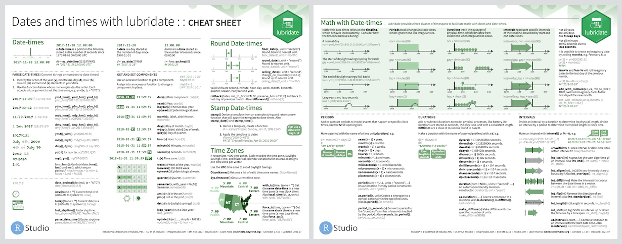
You have a pdf summary of the most important packages in the corresponding folder on campus
💻 It’s your turn
Try to perform the following exercises without looking at the solutions
📝 Define a variable that stores your age (called age) and another with your name (called name).
📝 Check with this variable age if it is NOT 60 years old or if it is called "Ornitorrinco" (you must obtain logical variables as a result).
📝 Why does the lower code give an error?
📝 Define another variable called siblings that answers the question “do you have siblings?” and another variable that stores your date of birth (called birth_date).
📝 Define another variable with your last name (called surname) and use glue() to have, in a single variable called full_name, your first and last name separated by a comma.
L2 : databases
Concatenating cells: vectors. First databases
Vectors: concatenation
When working with data, we often have columns that represent variables: we will refer to these as vectors, which are a concatenation of cells (values) of the same type (similar to a column in a table).
The simplest way to create a vector is with the c() function (c stands for concatenate), and you just need to input the elements within parentheses, separated by commas.
Consejo
An individual number x <- 1 (or x <- c(1)) is actually a vector of length one –> everything we know how to do with a number, we can do with a vector of numbers.
Vectors: concatenation

Numeric sequences
The most common type of vector is numeric, specifically, the well-known numeric sequences (e.g., the days of the month), used among other things, to index loops.
The seq(start, end) function allows us to create a [**numeric sequence]**{.hl-yellow} from a starting element to an ending one, advancing one by one.
Numeric sequences
A shortcut is the 1:n command, which returns the same as seq(1, n).
If the starting element is greater than the ending one, it understands that the sequence is in descending order.
Numeric sequences
Sometimes we may want to define a sequence with a specific length.
[1] 1.000000 9.166667 17.333333 25.500000 33.666667 41.833333 50.000000We might also want to generate a vector of n repeated elements.
String vectors
A vector is a concatenation of elements of the same type, but they don’t necessarily have to be numbers. Let’s create a sample sentence.
String vectors
What will happen if we concatenate elements of different types?
Note that since all elements must be of the same type, what R does is convert everything to text, violating the data integrity.
Operations with vectors
With numeric vectors, we can perform the same arithmetic operations as with numbers → a number is a vector (of length one).
What will happen if we add or subtract a value to a vector?
Adding vectors
Vectors can also interact with each other, so we can define, for example, vector sums (element by element).
Since the operation (e.g., a sum) is performed element by element, what will happen if we add two vectors of different lengths?
Comparing vectors
A very common operation is to ask questions of the data using logical conditions. For example, if we define a vector of temperatures…
Which days were below 22 degrees?
This will return a logical vector, depending on whether each element meets the given condition (of the same length as the vector being queried).
Comparing vectors
Logical conditions can be combined in two ways:
- Intersection: all concatenated conditions must be met (AND conjunction with
&) to returnTRUE.
- Union: it is enough for at least one condition to be met (OR conjunction with
|).
Getting elements
Another common operation is accessing or getting elements. The simplest way is to use the [i] operator (access the i-th element).
Since a number is just a vector of length one, this operation can also be applied using a vector of indices to select.
Consejo
To access the last element without worrying about its position, you can pass the vector’s length as the index x[length(x)].
Removing elements
Sometimes, instead of selecting, we may want to remove elements. This is done with the same operation but using negative indexing: the opetator [-i] «un-select» the i-th element
[1] "hi" "how" "are" "you" "?" [1] "hi" "are" "you" "?" In many cases, we want to select or remove elements based on logical conditions, depending on the values, so we will pass the condition itself as the index (remember, x < 2 returns a logical vector).
Stats operations
We can also make use of statistical operations, such as sum(), which, given a vector, returns the sum of all its elements.
What happens when a data point is missing?
Stats operations
As we’ve mentioned, logical values are internally stored as 0 and 1, so we can use them in arithmetic operations.
For example, if we want to find out the number of elements that meet a condition (e.g., less than 3), those that do will be assigned a 1 (TRUE), and those that don’t will get a 0 (FALSE). Therefore, summing the logical vector will give us the number of elements that meet the condition.
Stats operations
Another common operation that can be useful is the cumulative sum with cumsum(), which, given a vector, returns a vector where each element is the sum of the first, the first plus the second, the first plus the second plus the third, and so on.
What happens when a data point is missing?
In the case of the cumulative sum, what happens is that from that point onward, all subsequent accumulated values will be missing.
Stats operations
Another common operation that can be useful is the difference (with delay) with diff() which, given a vector, returns a vector with the second minus the first, the third minus the second, the fourth minus the third…and so on.
Stats operations
Other common operations are mean, median, percentiles, etc.
- mean: centrality measure that consists of adding all the elements and dividing by the number of elements added. The best known but the least robust: given a set, if outliers (very large or very small values) are introduced, the mean is very easily perturbed.
Stats operations
Other common operations are mean, median, percentiles, etc.
- Median: measure of centrality that consists of ordering the elements and keeping the one that occupies the middle.
Sorting vectors
Finally, a common action is to know sort values:
sort(): returns the sorted vector. By default from smallest to largest but withdecreasing = TRUEwe can change it.
[1] 7 20 23 25 33 41 65 77 81[1] 81 77 65 41 33 25 23 20 7💻 It’s your turn
Try to perform the following exercises without looking at the solutions
- Exercise 1
- Exercise 2
- Exercise 3
- Exercise 4
- Exercise 5
- Exercise 6
- Exercise 7
- Exercise 8
- Exercise 9
- Exercise 10
- Exercise 11
- Exercise 12
📝 Define the vector x as the concatenation of the first 5 odd numbers. Calculate the length of the vector
📝 Access the third element of x. Access the last element (regardless of length, a code that can always be executed). Delete the first element.
📝 Get the elements of x greater than 4. Calculate the vector 1/x and store it in a variable.
📝 Create a vector representing the names of 5 people, one of whom is unknown.
📝 Find from the vector x of exercises above the elements greater (strictly) than 1 and less (strictly) than 7. Find a way to find out if all the elements are positive or not.
📝 Given the vector x <- c(1, -5, 8, NA, 10, -3, 9), why does its mean return not a number but what is shown in the code below?
📝 Given the vector x <- c(1, -5, 8, NA, 10, -3, 9), extract the elements occupying the locations 1, 2, 5, 6.
📝 Given the x vector of the previous exercise, which ones have a missing data? Hint: the is.something() functions check if the element is of type something (press tab).
📝 Define the vector x as the concatenation of the first 4 even numbers. Calculate the number of elements of x strictly less than 5.
📝 Calculate the vector 1/x and obtain the ordered version (from smallest to largest) in the two possible ways
More with string variables
Although we cannot do arithmetic operations with them, some operations we can do with the text strings will be important.
For that we will use in the future the {stringr} package (within the same {lubridate} “universe of packages”, which we will talk about later).
First databases
When analyzing data we usually have several variables for each individual: we need a “table” to collect them. The most immediate option is matrices: concatenation of variables of same type and equal length.
Imagine we have heights and weights of 4 people. How to create a dataset with the two variables?
First databases
We can also build the matrix by rows with the rbind() function (concatenate - bind - by rows - r), although it is recommended to have each variable in column and individual in row as we will see later.
- We can “view” the matrix with
View(matrix).
First databases
We can also “flip” (transposed matrix) with t().
First databases
In some cases we will want to get the total data for an individual (a particular row but all columns) or the values of a whole variable for all individuals (a particular column but all rows). To do so, we leave one of the indexes unfilled.
First databases
We can also define a matrix from a numeric vector, rearranging the values in the form of a matrix (knowing that the elements are placed by columns).
Matrix operations
With matrices it is the same as with vectors: when we apply an arithmetic operation we do it element by element
Matrix operations
We can also perform operations by columns/rows without loops with the apply() function, and we will indicate as arguments
- the matrix
- the sense of the operation (
MARGIN = 1for rows,MARGIN = 2for columns) - the function to apply
- extra arguments needed by the function
💻 It’s your turn
Try to perform the following exercises without looking at the solutions
📝 Modify the code below to define an x matrix of ones, with 3 rows and 7 columns.
📝 To the above matrix, add 1 to each number in the matrix and divide the result by 5. Then calculate its transpose
📝 Why does the code below return such a warning message?
📝 Define the matrix x <- matrix(1:12, nrow = 4). Then get the data of the first individual, the data of the third variable, and the element (4, 1).
📝 Define a matrix of 2 variables and 3 individuals such that each variable captures the height and age of 3 persons, so that the age of the second person is unknown (absent). Then calculate the mean of each variable (we should get a number!).
Second attempt: data.frame
Arrays have the same problem as vectors: if we put together data of different types, it data integrity is compromised as it converts them (see the code below: the ages and the TRUE/FALSE are converted to text).
Second attempt: data.frame
In order to work with variables of different type we have in R what is known as data.frame: concatenation of variables of equal length but which can be of different type.
Second attempt: data.frame
Since a data.frame is already an attempt at a database the variables are not mere mathematical vectors: they have a meaning and we can (we must) give them names that describe their meaning.
Second attempt: data.frame
We have our first data set! (strictly speaking we can’t talk about a database but for the moment it looks like one). You can visualize it by typing its name in console or with View(table).

Get variables
If we want to access its elements, being again tabulated data, we can access as in the matrices (not recommended): again we have two indexes (rows and columns, leaving free the one we don’t use)
  ages single names birth_date
2 24 NA laura 1992-04-01[1] "javi" "laura" "lucía"[1] 24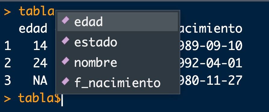
But it also has the advantages of a database : we can access the variables by name (recommended since the variables can change position and now they have a meaning), putting the name of the table followed by the symbol $ (with the tab, a menu of columns to choose from will appear).
Ask functions
names(): shows us the variable names
Add a variable
If we have one already created and we want to add a column it is as simple as using the data.frame() function we have already seen to concatenate the column. Let’s add for example a new variable, the number of siblings of each individual.
Last attempt: tibble
Tables in data.frame format have some limitations. The main one is that does not allow recursion: imagine that we define a database with heights and weights, and we want a third variable with the BMI.
Error in data.frame(height = c(1.7, 1.8, 1.6), weight = c(80, 75, 70), : object 'weight' not foundHereafter we will use the tibble (enhanced data.frame) format from the {tibble} package.
Last attempt: tibble
data_tb <-
  tibble("height" = c(1.7, 1.8, 1.6), "weight" = c(80, 75, 70), "BMI" = weight / (height^2))
class(data_tb)
[1] "tbl_df" "tbl" "data.frame"# A tibble: 3 × 3
height weight BMI
<dbl> <dbl> <dbl>
1 1.7 80 27.7
2 1.8 75 23.1
3 1.6 70 27.3Las tablas en formato tibble nos permitirá una gestión más ágil, eficiente y coherente de los data, con 4 ventajas principales:
- Metainformation: if you look at the header, it automatically tells us the number of rows and columns, and the type of each variable
- Recursivity: allows you to define the variables sequentially (as we have seen)
Last attempt: tibble
- Consistency: if you access a column that does not exist, it warns you with a warning
- By rows: create by rows (copy and paste from a table) with
tribble().
Consejo
The {datapasta} package allows us to copy and paste tables from web pages and simple documents as a tribble. See more in https://milesmcbain.github.io/datapasta/articles/how-to-datapasta.html#pasting-a-table-as-a-formatted-tibble-definition-with-tribble_paste
In summary…
- Each cell can be of a different type: numbers, text, dates, logical values, etc. A [vector is a concatenation of cells]{. hl-yellow} (the future columns of our tables) –> In
Rby default operations are done element to element.
- A matrix allows us to concatenate variables of the SAME type and SAME length –> tabular data.
- A data.frame allows us to concatenate variables of DIFFERENT type and SAME length –> we will use tibble as an enhanced database option.
💻 It’s your turn
Try to perform the following exercises without looking at the solutions
📝 Load from the {datasets} package the airquality dataset (New York air quality variables from May through September 1973). Is the airquality dataset of type tibble? If not, convert it to tibble (look in the package documentation at https://tibble.tidyverse.org/index.html).
📝 Once converted to tibble get the name of the variables and the dimensions of the data set. How many variables are there? How many days have been measured?
📝 Filter only the data for the month of August. How to tell it that we want only the rows that meet a specific condition?
📝 Select those data that are not from July or August.
📝 Modify the following code to keep only the ozone and temperature variables (no matter what position they are).
📝 Select the temperature and wind data for August.
🐣 Case study I
In the {datasets} package (already installed by default) we have several datasets and one of them is airquality. Below I have extracted 3 variables from that dataset (note that it is done with data$variable, that dollar will be important in the future).The data captures daily measurements (n = 153 observations) of air quality in New York, from May to September 1973. Six 6 variables were measured: ozone levels, solar radiation, wind, temperature, month and day.
Try to answer the questions posed in the workbook
🐣 Case study II
We will consider the surveys.RData file in which we have all poll surveys for Spain from 1982 to 2019.
# A tibble: 139,944 × 8
   date_elec  pollster field_date_from field_date_to exit_poll  size party
   <date>     <chr>    <date>          <date>        <lgl>     <dbl> <chr>
 1 1982-10-28 PSOE     1982-10-28      1982-10-28    TRUE      85300 UCD
 2 1982-10-28 PSOE     1982-10-28      1982-10-28    TRUE      85300 PSOE
 3 1982-10-28 PSOE     1982-10-28      1982-10-28    TRUE      85300 PCE
 4 1982-10-28 PSOE     1982-10-28      1982-10-28    TRUE      85300 AP
 5 1982-10-28 PSOE     1982-10-28      1982-10-28    TRUE      85300 CIU
 6 1982-10-28 PSOE     1982-10-28      1982-10-28    TRUE      85300 PA
 7 1982-10-28 PSOE     1982-10-28      1982-10-28    TRUE      85300 EAJ-PNV
 8 1982-10-28 PSOE     1982-10-28      1982-10-28    TRUE      85300 HB
 9 1982-10-28 PSOE     1982-10-28      1982-10-28    TRUE      85300 ERC
10 1982-10-28 PSOE     1982-10-28      1982-10-28    TRUE      85300 EE
# ℹ 139,934 more rows
# ℹ 1 more variable: estimation <dbl>
Try to answer the questions posed in the workbook
L3: if-else and Quarto
Flow structures: if-else and loops. Functions in R. Quarto
Flow structures
A flow or control structure consists of a series of commands oriented to decide the path that your code must follow
If condition A is met, what happens?
What if B happens?
How can I repeat the same expression (depending on a variable)?
If you have programmed before, you may be familiar with what are known as conditional structures such as if (bla bla) {...} else {...} or loops for/while (to be avoided whenever possible).
If
One of the most famous control structures are those known as conditional structures if.
IF a set of conditions is met (TRUE), then execute whatever is inside the curly brackets.
For example, the structure if (x == 1) { code A } what it will do is execute code A in braces but ONLY IF the condition in brackets is true (only if x is 1). In any other case, it will do nothing
If
Our conditional structure will do the following: if there is a minor, it will print a message.
If
In case the conditions are not true inside if() (FALSE), nothing happens.
We get no message because the condition all(ages >= 18) is not TRUE, so it does not execute anything.
If-else
The structure if (condition) { code A } can be combined with an else { code B }: when the condition is not checked, it will [execute the alternative code B]{. hl-yellow} inside else { }, allowing us to decide what happens when it is satisfied and when it is not
If-else
Esta estructura if - else puede ser anidada: imagina que queremos ejecutar un código si todos son menores; si no sucede, pero todos son mayores de 16, hacer otra cosa; en cualquier otra cosa, otra acción.
if (all(ages >= 18)) {

  print("All of them are of legal age")

} else if (all(ages >= 16)) {
print("There is a minor but all of them are greater or equal to 16 years old")
} else { print("There are any persons under 16 years of age") }[1] "There are any persons under 16 years of age"Tip
You can collapse the structures by clicking on the left arrow in your script.
If-else vectorized
This conditional structure can be vectorized (in a single line) with if_else() (from the {dplyr} package), whose arguments are
the condition to evaluate
what happens when it is met and when not
an optional argument for when the condition to evaluate is
NA
We will label without are greater/lesser and an unknown when we don’t know.
[1] "unknown"   "minor"     "minor"     "legal age" "legal age" "legal age"
[7] "legal age" "legal age" "legal age"
In R base there is ifelse(): it does not let you specify what to do with the absent ones but allows you to specify different types of data in TRUE and FALSE.
💻 It’s your turn
Try to perform the following exercises without looking at the solutions
📝 What will be the output of the following code?
📝 What will be the output of the following code?
📝 Modify the code below so that, when the square root of a number cannot be verified to be less than 2, it returns -1.
📝 What are the values of x and y of the lower code for z <- 1, z <- -1 and z <- -5?
📝 What will happen if we execute the code below?
📝 From the {lubridate} package, the hour() function returns the time of a given date, and the now() function returns the date and time of the current time. With both functions, have cat() (cat()) print “good night” only after 21:00.
Communicate: rmd and Quarto
One of the main strengths of R is the easiness to generate reports, books, webs, notes and even slides (this same material for example). To do this, install before
- the
{rmarkdown}package (to generate.rmdfiles)
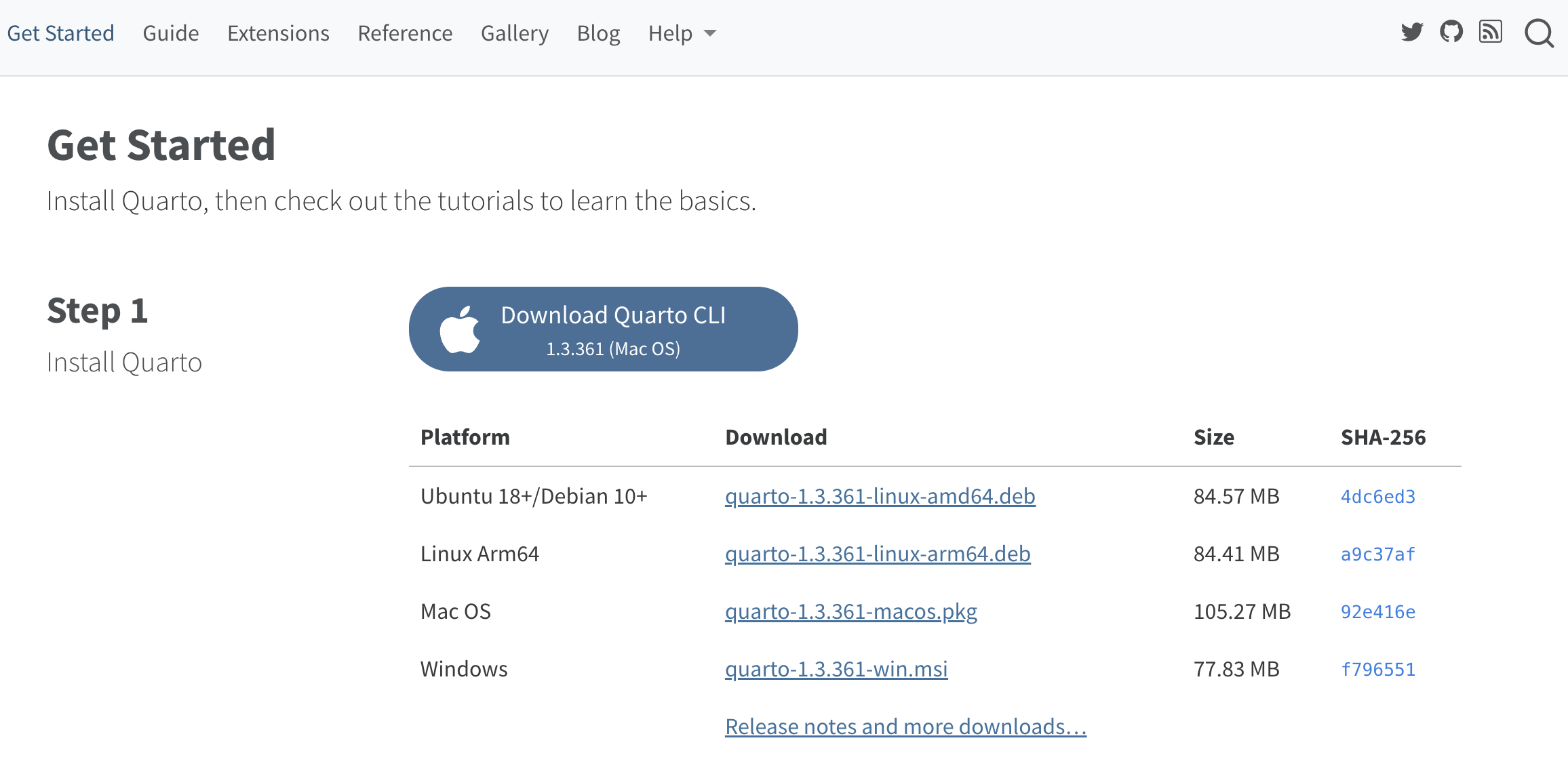
- install Quarto (if you already knew
R, the “new”.rmdnow as.qmd)
Communicate: rmd and Quarto
So far we have only programmed in scripts (.R files) within projects, but in many occasions we will not work alone and we will need to communicate the results in different formats:
- notes (for ourselves)
- slides
- web
- reports
For all this we will use Quarto (see more in https://ivelasq.quarto.pub/intro-to-quarto/)
Communicate: rmd and Quarto
The .qmd (or .rmd before) extension files will allow us to easily combine:- Markdown:
- typed language that allows us to create simple content (wordpress type, with text, bold, cursives, etc) with a readable layout.
- [Math (latex)]{. hl-yellow}: language for writing mathematical notation such as \(x^2\) or \(\sqrt{y}\) or \(\int_{a}^{b} f(x) dx\).
- Code and outputs: we can not only show the final step but also the code you have been doing (in
R,Python,C++,Julia, …), with code boxes called CHUNKS.
- Images, graphs, tables, styles (css, js), etc.
Communicate: rmd and Quarto
The main advantage of making this type of material in Quarto/Rmarkdown is that, by doing it from RStudio, you can generate a report or presentation without leaving the programming environment in which you are working. This way you can analyze the data, summarize it and at the same time communicate it with the same tool.
Recently the RStudio team developed Quarto, an improved version of Rmarkdown (.qmd files), with a slightly more aesthetic and simpler format. You have all the documentation and examples at https://quarto.org/
Quarto examples
Images obtained from https://ivelasq.quarto.pub/intro-to-quarto/#/working-with-the-rstudio-visual-editor
Our first report
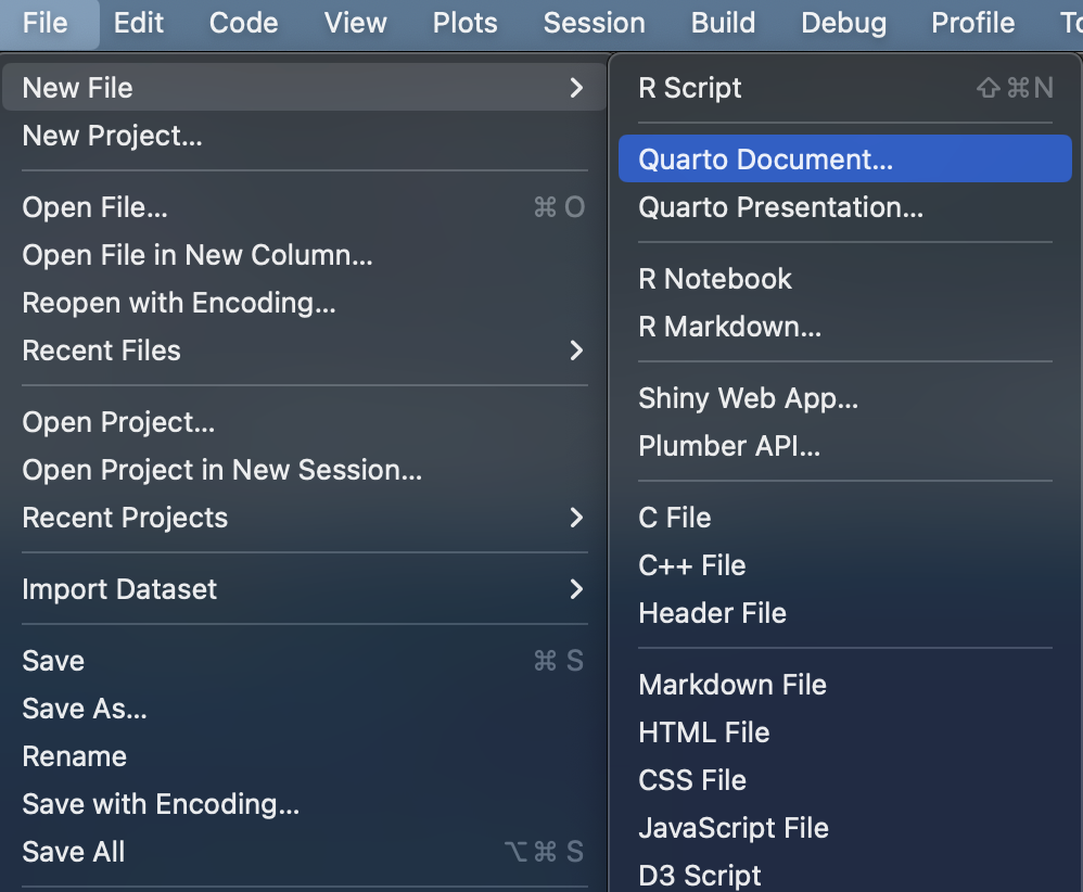
We are going to create the first rmarkdown file with Quarto with extension .qmd. For this we will only need to click on
File << New File << Quarto Document
Our first report

After doing so, several output format options:
.pdffile.htmlfile (recommendable): dynamic document, allows user interaction, like a “web page”..docfile (not recommended).
For the moment we will leave the default HTML format checked, and we will write the title of our document. After that we will have our file .qmd (it is no longer an .R script like the ones we have opened so far).
Our first report
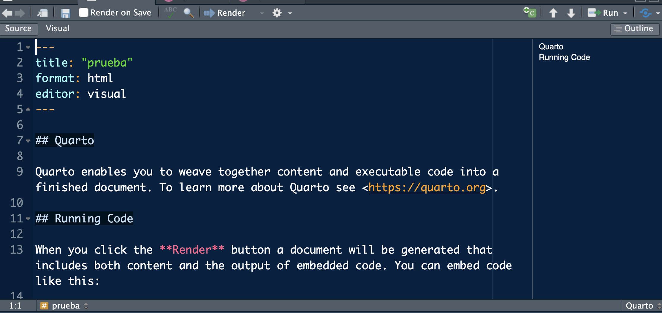
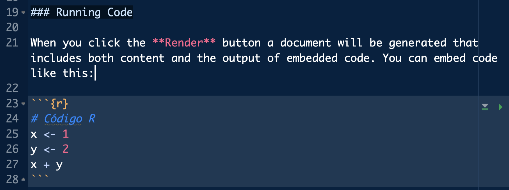
You should have something similar to the image capture with two editing modes: Source (with code, the recommended option until you master it) and Visual (more like a blog).
To run the WHOLE document you must click Render on Save and hit save.
Quarto output format
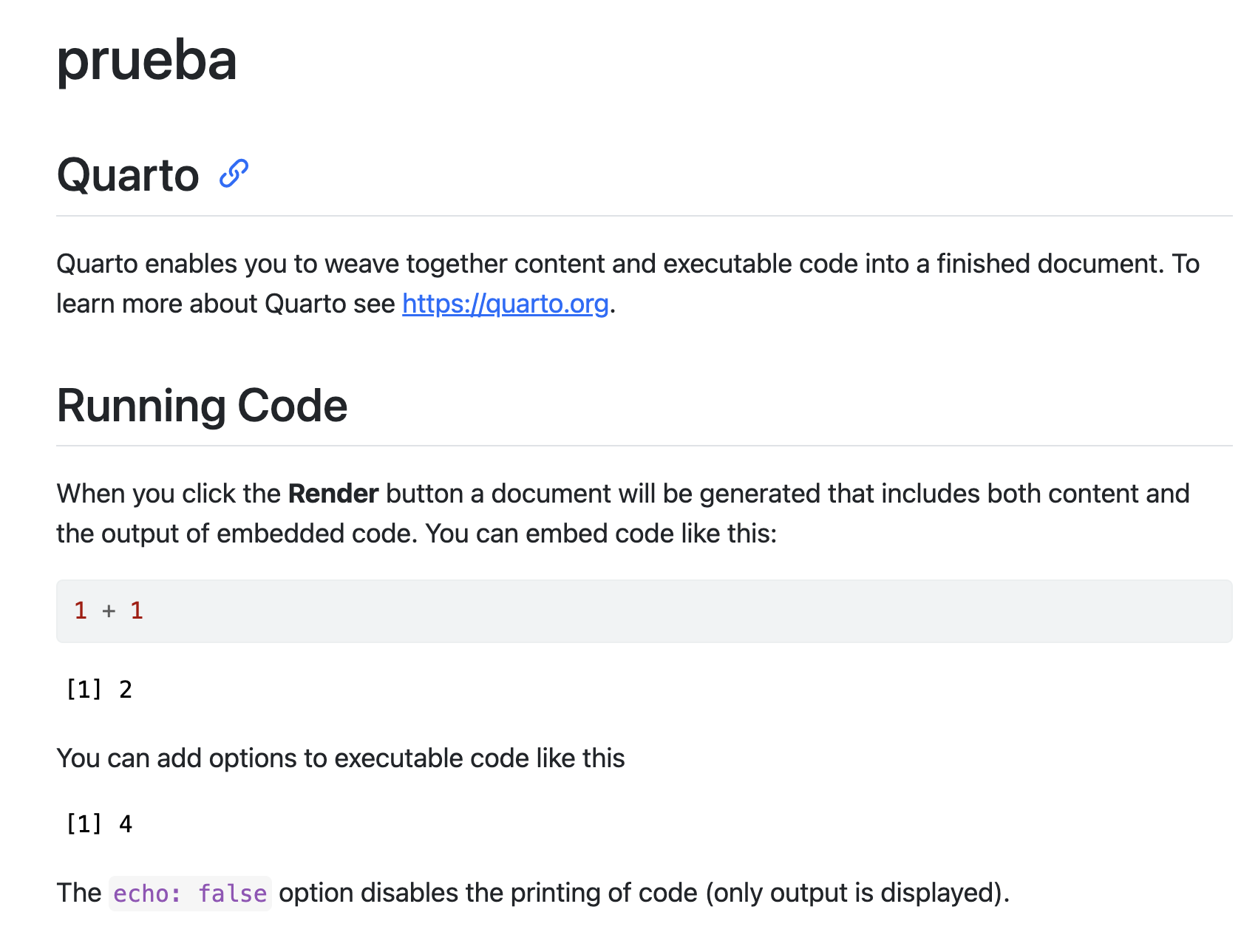
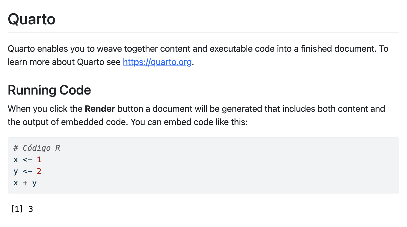
You should have obtained an html output similar to this (and a html file has been generated on your computer).
Editor: source vs visual
As indicated, you have two ways of working: with pure code and something similar to a Notion (blog).
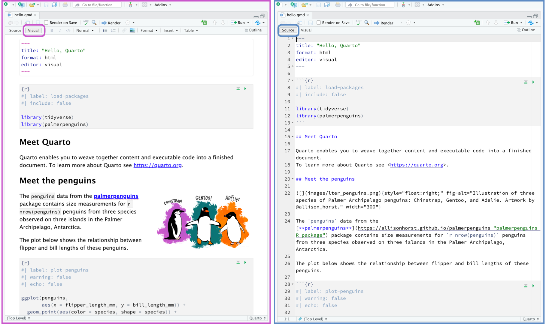
Image retrieved from https://ivelasq.quarto.pub/intro-to-quarto/#/working-with-the-rstudio-visual-editor
Our first report

A .qmd file is basically divided into three parts:
Header: the part you have at the beginning between
---.[Text]{. hl-yellow}: which we can format and enhance with bold (written as bold, with double asterisk at the beginning and end), italics (cursive, with underscore at the beginning and end) or highlight function or variable names from R. You can add equations like \(x^2\) (I have written
$x^2$, between dollars).R code
Header
The header is in YAML format and contains the metadata of the document.
titleandsubtitle: the title/subtitle of the documentauthor: author of the documentformat: output format (we can customize)theme: if you have any style filetoc: if you want index or nottoc-location: index positiontoc-title: index title
editor: if you are in visual or source mode.
Text
Regarding typing there is only one important thing: unless we indicate otherwise, EVERYTHING we are going to type is (normal) text; no R code.
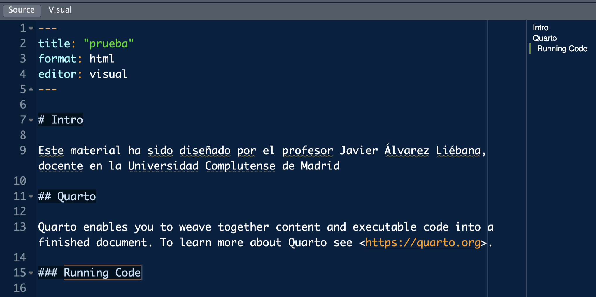
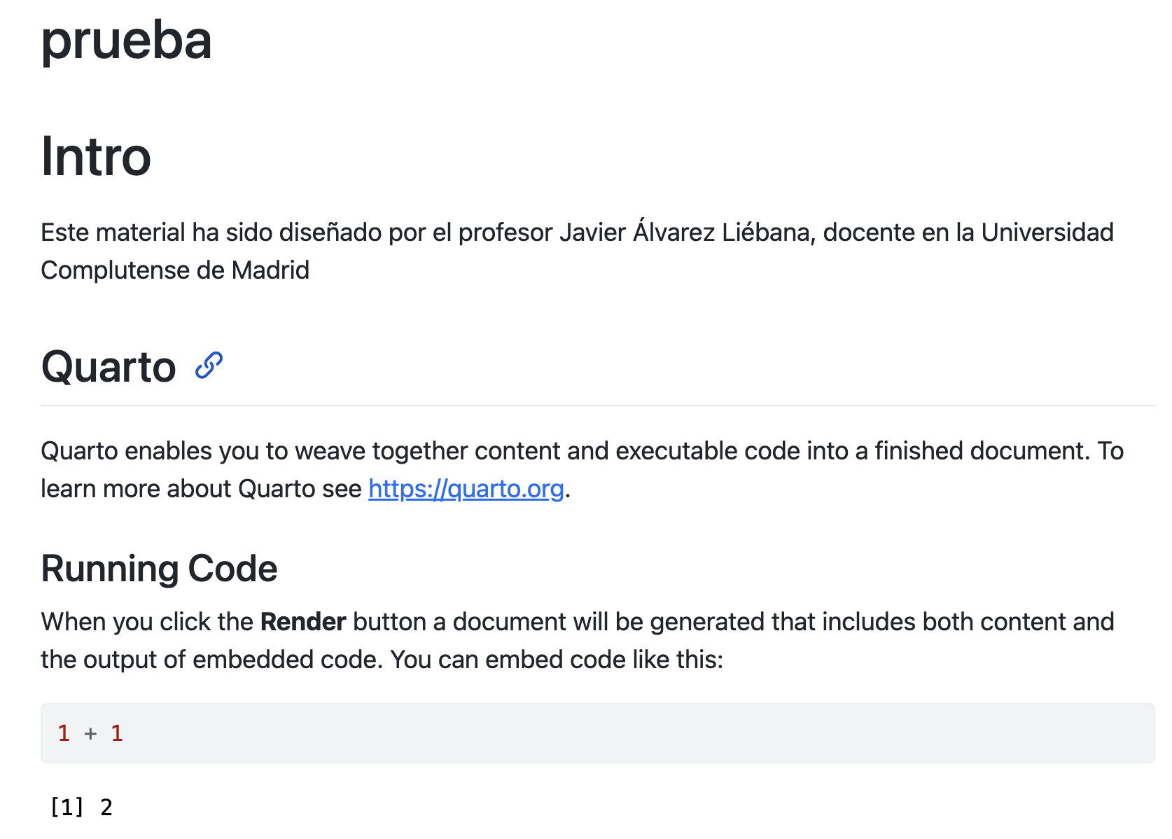
We are going to start by writing a section at the beginning (# Intro and behind it, for example, the sentence
This material has been designed by Professor Javier Álvarez Liébana, professor at the Complutense University of Madrid
In addition to the Running Code we will add a # pad: the outside-chunks pads will help us create epigraphs (sections) in the document.
Index
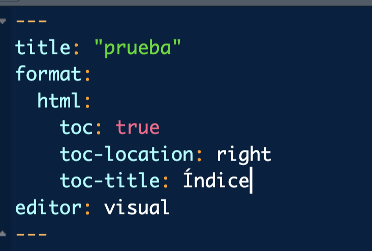
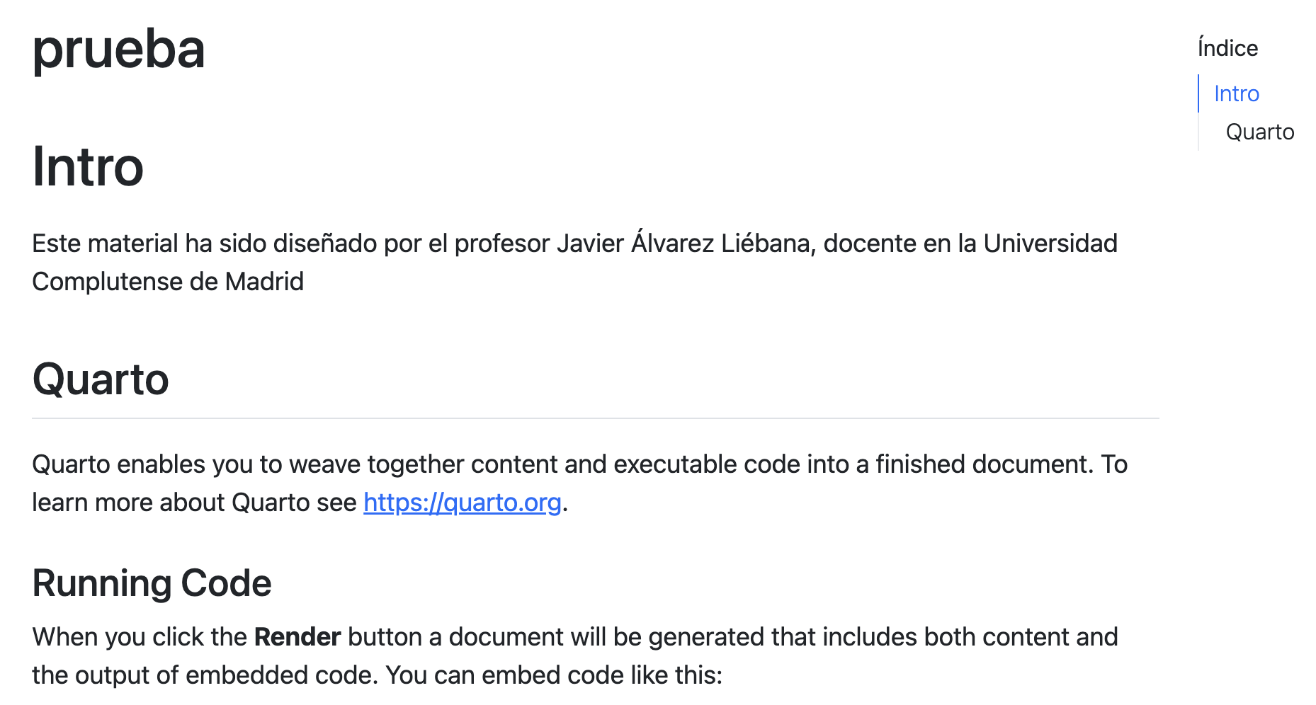
To make the index capture those sections we will modify the header of the file as shown in the image (you can change the location of the index and the title if you want to test).
Text
Let’s customize the text a bit by doing the following:
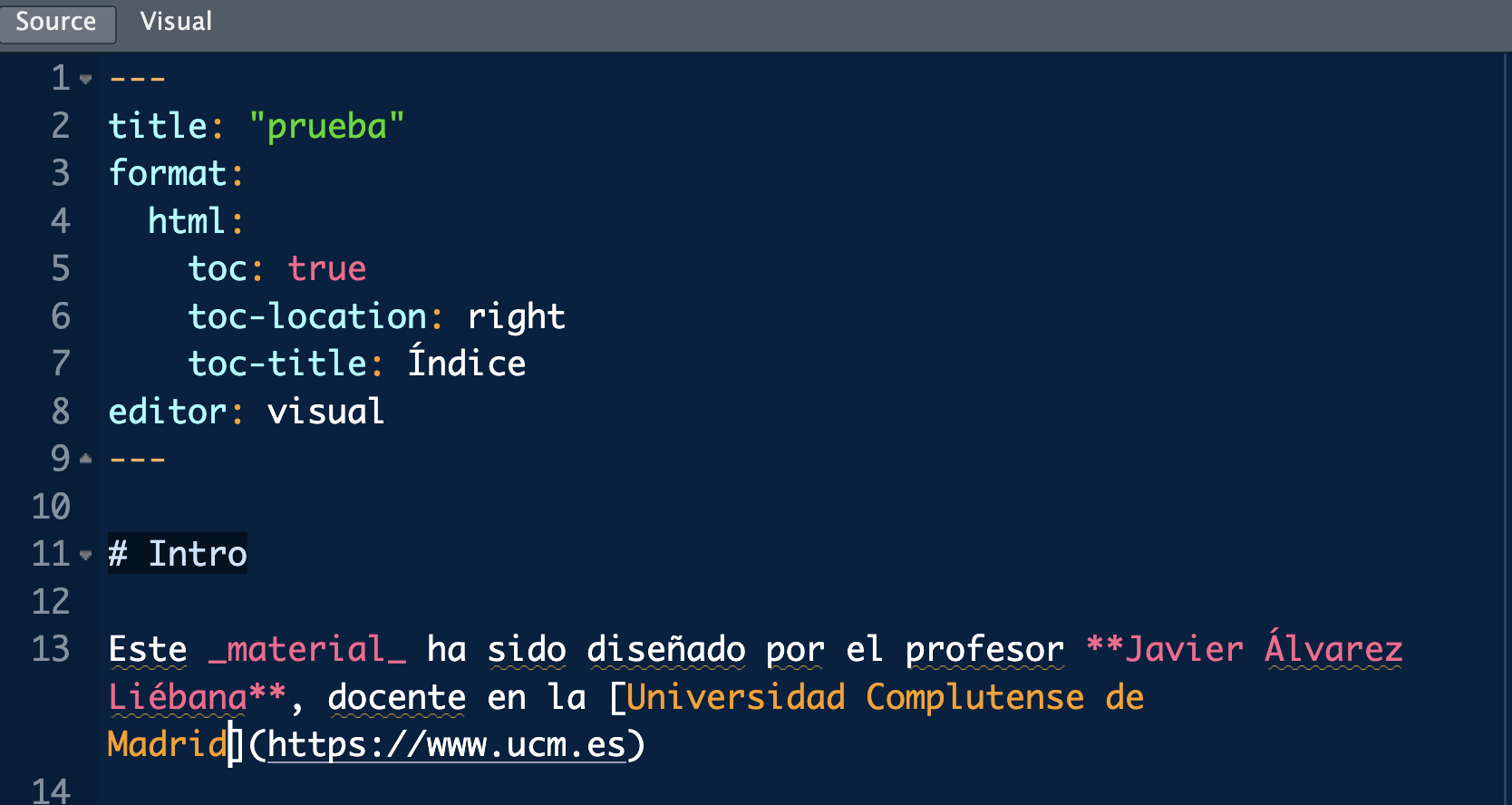
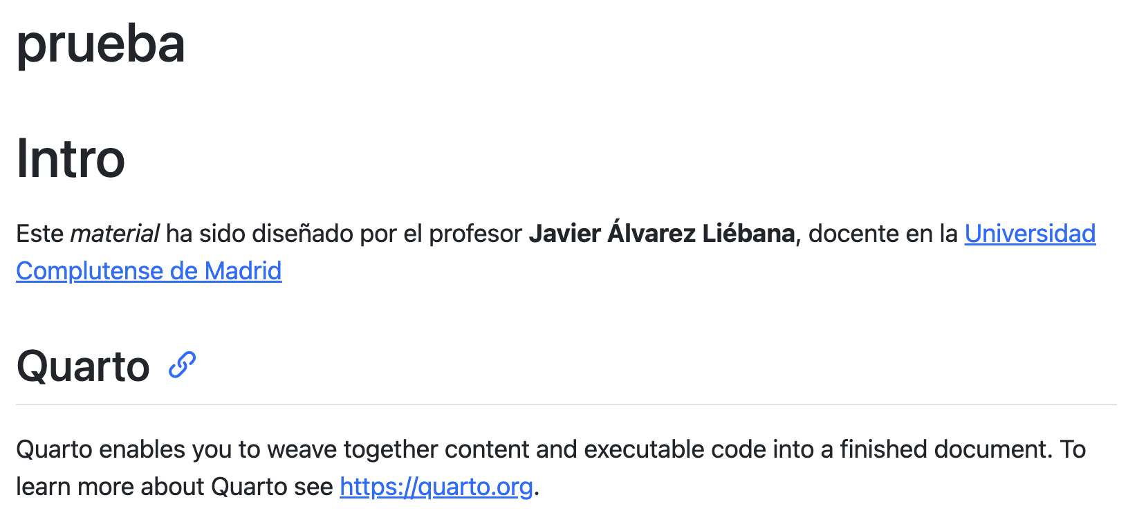
We will add bold to the name (putting ** at the beginning and at the end).
We will add cursive to the word material (putting _ at the beginning and at the end).
We will add a link https://www.ucm.es, associating it to the name of the University. To do this we put the title in square brackets and just behind the link in brackets
[“Universidad Complutense de Madrid”](https://www.ucm.es).
Code
To include R code we must create our code boxes called chunks: high in the path in our markdown text where we can include code from almost any language (and its outputs).

To include one you must go header as follows you have a shortcut Command + Option + I (Mac) or Ctrl + Shift + I (Windows)
Code
Inside this box (which now has a different color in the document) write code R as we have been doing so far in the scripts.
Running chunks
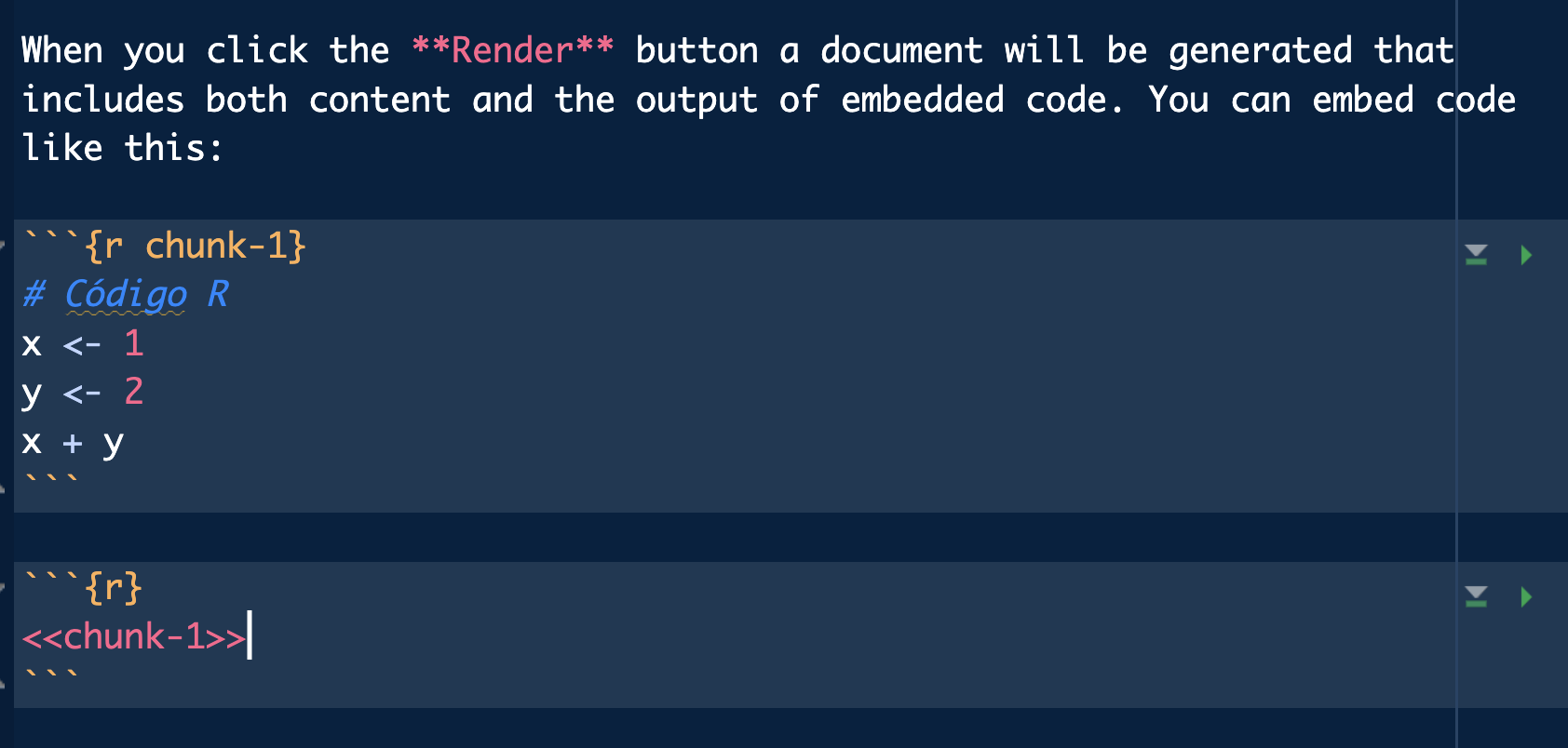
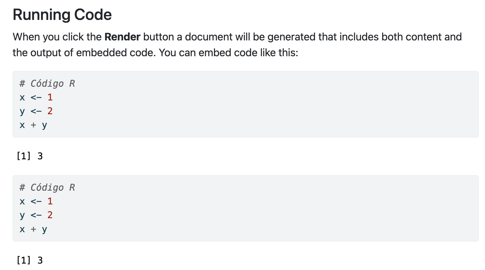
Chunks can have a name or tag, so that we can reference them again to avoid repeating code.
Running chunks
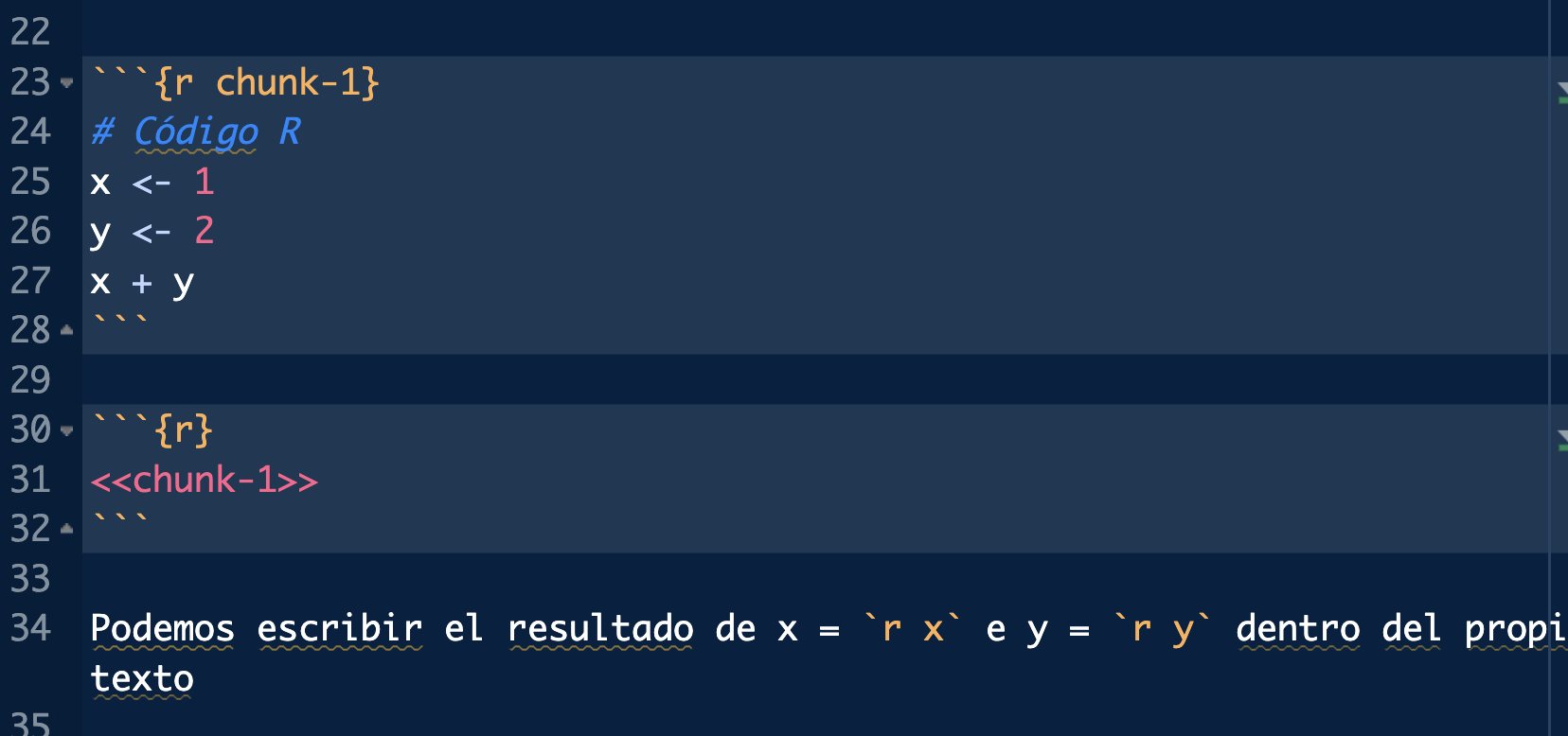
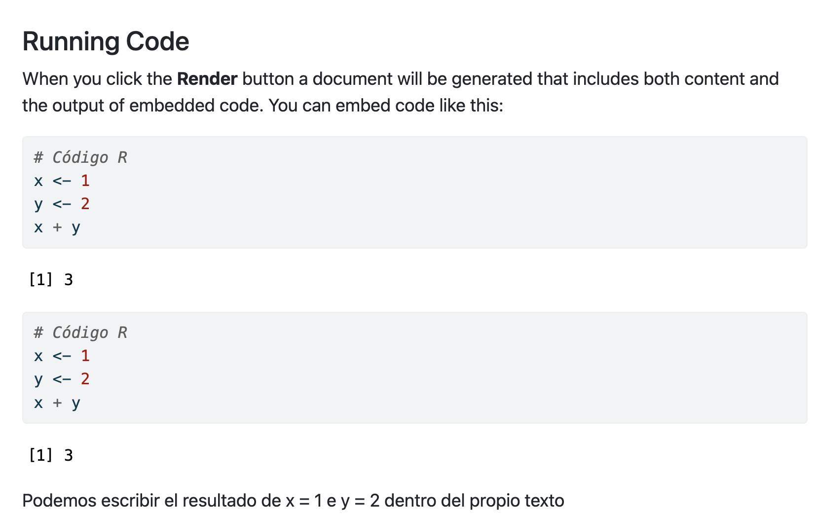
In each chunk there are two buttons:
play button: activates the play and exit of that particular chunk (you can view it within your own
RStudio)rewind button: activates the play and exit of all chunks up to that one (without reaching it).
In addition we can include R code inside the text line (instead of displaying the text x execute the R code displaying the variable).
Customizing chunks
The chunks can be customized with options at the beginning of the chunk preceded by #|:
#| echo: false: execute code and show result but does not display code in the output. hl-red} on output.#| include: false: executes code but does not display result and does not display code on output.#| eval: false: [does not execute code]{. hl-red}, does not display result but does display code on output.#| message: false: executes code but does not display output messages.#| warning: false: runs code but does not display warning messages.#| error: true: runs code and allows errors displaying the error message in the output.

These options can be applied chunk by chunk or set globally with knitr::opts_chunk$set() at the beginning of the document (within a chunk).
Customizing chunks
If we want to apply the option to all chunks by default we must include it at the end of the header, as run options
Organizing
In addition to text and code we can enter the following:
Equations: you can also add equations like \(x^2\) (I have written
$x^2$, the equation between dollars).[Lists]{. hl-yellow}: you can itemize elements by putting
* Step 1: ... *Step 2: ...Cross-references: you can tag parts of the document (the tag is constructed with
{#section-name}) and then call them with[Section](@section-name).
Figures and images

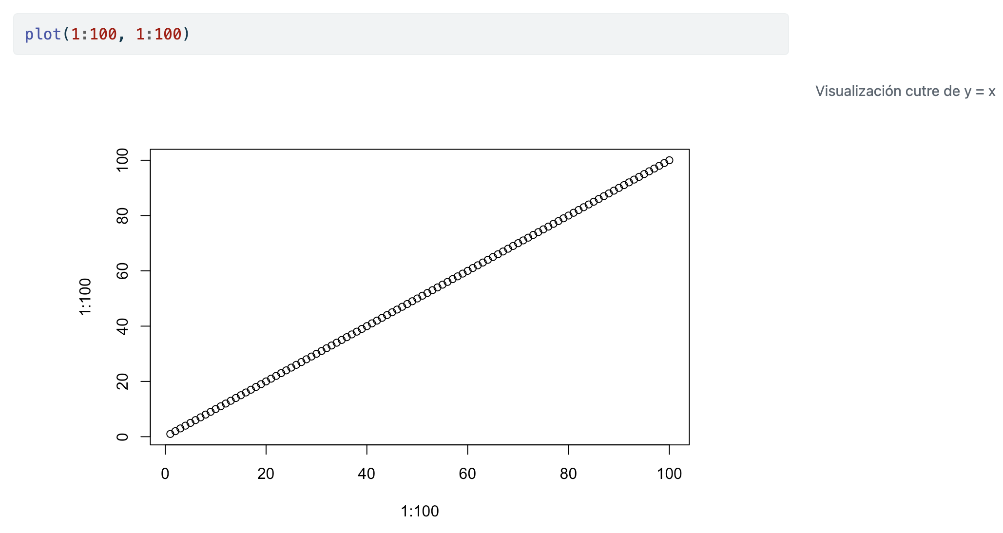
Finally, we can also add captions to graphics or images by adding #| fig-cap: "...".
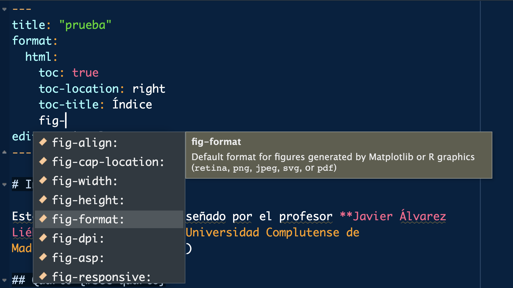
Notice that the caption is in the margin (for example). You can change it by entering header settings (everything about figures starts with fig-, and you can see the options by tabbing). You have more information at https://quarto.org/
Styles
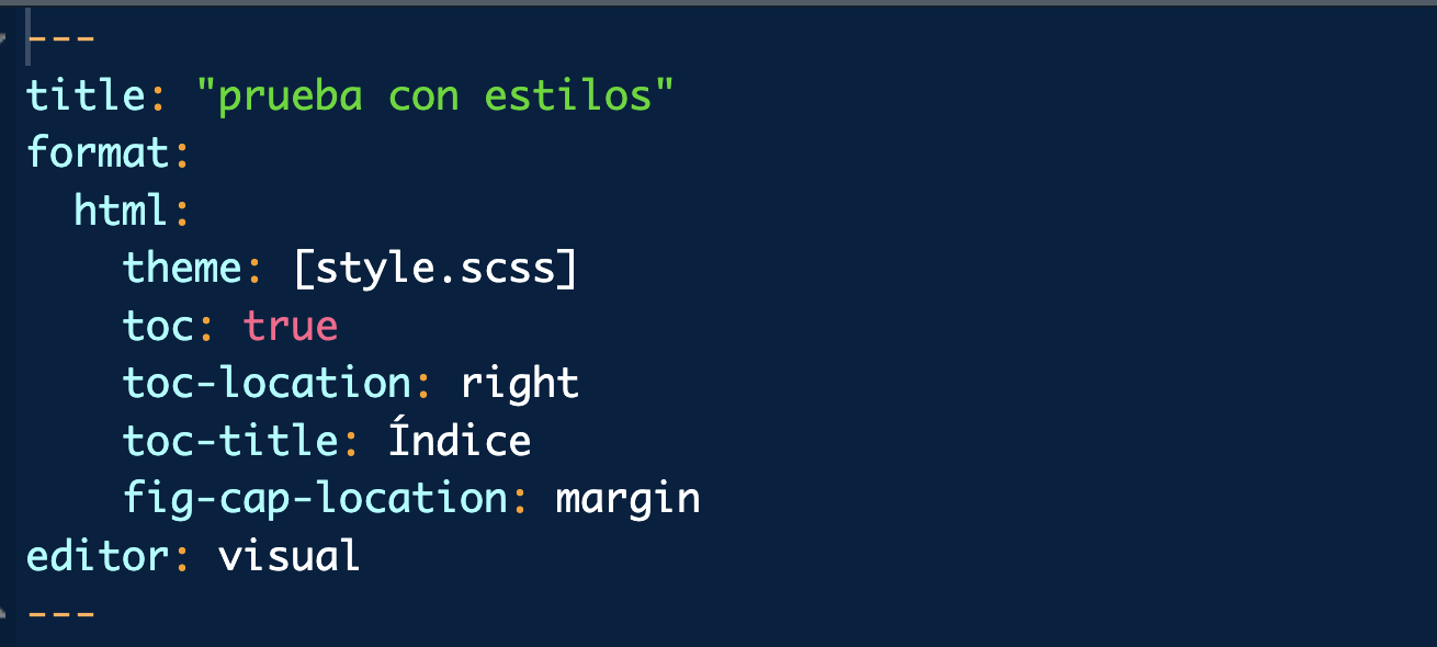
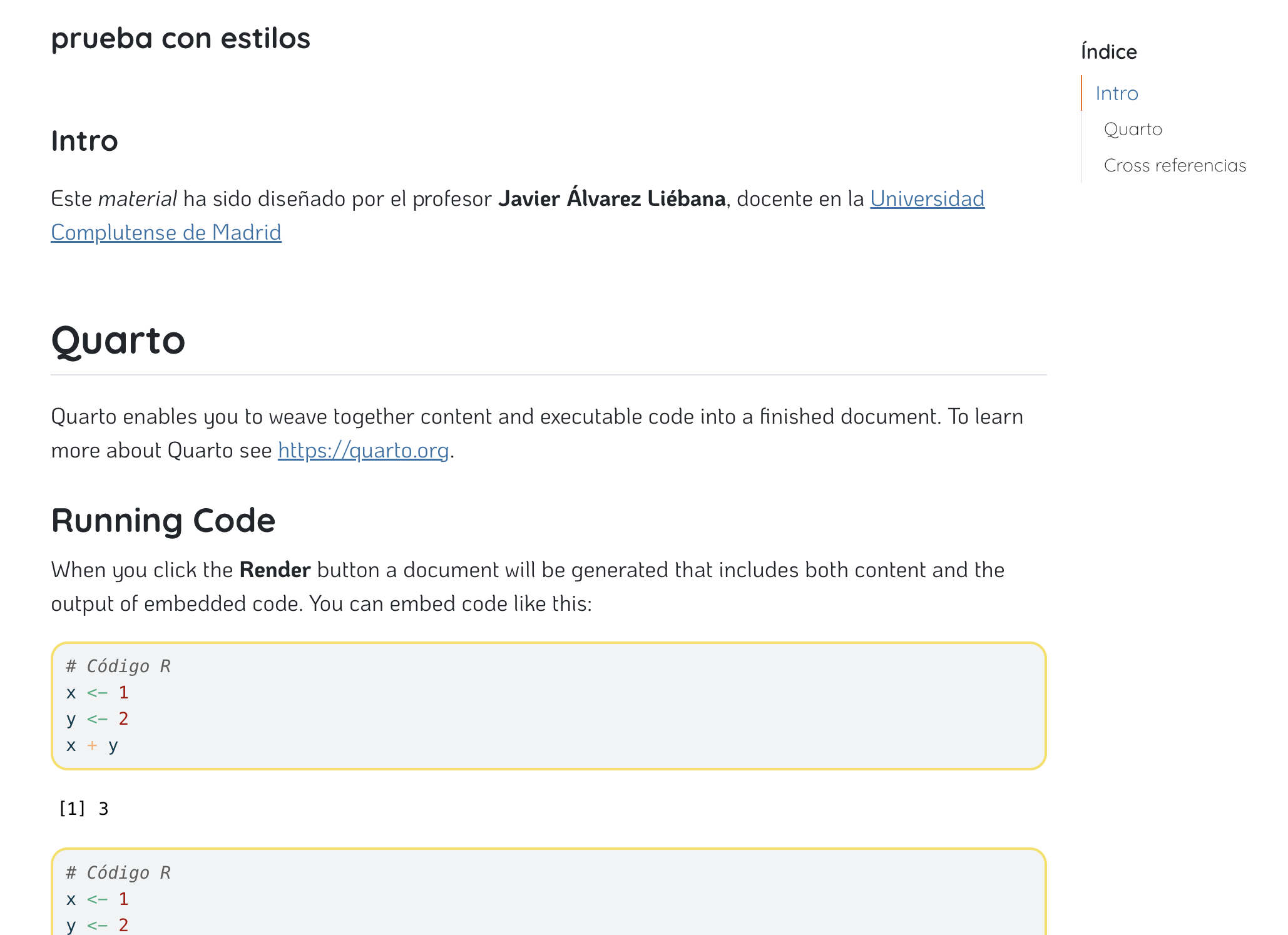
Finally you can add a custom theme including a style file (.scss or .css file). I have left one for you at https://github.com/dadosdelaplace/docencia-R-master-bio-2324/tree/main/material.
Important
The style file must be in the same folder as the .qmd file.
Styles
You can also do it in a simple way adding a bit of HTML to the text. For example, to customize the color of a text it goes between square brackets and right after the text, between braces, the style options
This word is red …
… and this is green in bold
Revealjs
You can add some “animations” using what is known as Revealjs (javascript), specifying it in the header and using blocks of that language delimited by ::: at the beginning and end, and the word of the “tool” to use. For example {.incremental} transitions the elements.
- I
- am
- Javi
Call blocks
You can also use the callout-blocks which by default are note, tip, warning, caution and important (although you can create and customize them). To do this, just use ::{.callout-type} and the type you want to use
:::{.callout-tip}

Note that there are five types of callouts, including:
`note`, `tip`, `warning`, `caution`, and `important`.

:::
Consejo
Note that there are five types of callouts, including: note, tip, warning, caution, and important.
Peligro
Use them wisely, sometimes a lot of aesthetic resources can be dizzying.
Multiple columns layout
With :::: columns we can define a layout of multiple columns where each one is defined by ::: {.column width=“65%”} something :::, indicating next to the percentage how much you want each column to occupy (be careful not to leave spaces!).
:::: columns
::: {.column width="65%"}
This is how to define a vector
:::
::: {.column width="35%"}
x <- c(1, 2, 3)
x
:::
::::
Non-R code
In addition {reticulate} allows us to create python chunks inside a Quarto in R (see https://quarto.org/docs/computations/python.html to create jupyter notebooks directly from Quarto).
🐣 Case study I: flow structures
To practice control structures we are going to perform a simulation exercise
Try to answer the questions posed in the workbook
🐣 Case study II: functions
Define a function called temperature_converter that, given a temperature in Fahrenheit, Celsius or Kelvin, converts it to any of the others
Try to answer the questions posed in the workbook
🐣 Case study III: mock task
Let’s perform a small simulation before delivery using the starwars dataset from the {dplyr} package.

🐣 Case study III: mock task
# A tibble: 87 × 14
   name     height  mass hair_color skin_color eye_color birth_year sex   gender
   <chr>     <int> <dbl> <chr>      <chr>      <chr>          <dbl> <chr> <chr>
 1 Luke Sk…    172    77 blond      fair       blue            19   male  mascu…
 2 C-3PO       167    75 <NA>       gold       yellow         112   none  mascu…
 3 R2-D2        96    32 <NA>       white, bl… red             33   none  mascu…
 4 Darth V…    202   136 none       white      yellow          41.9 male  mascu…
 5 Leia Or…    150    49 brown      light      brown           19   fema… femin…
 6 Owen La…    178   120 brown, gr… light      blue            52   male  mascu…
 7 Beru Wh…    165    75 brown      light      blue            47   fema… femin…
 8 R5-D4        97    32 <NA>       white, red red             NA   none  mascu…
 9 Biggs D…    183    84 black      light      brown           24   male  mascu…
10 Obi-Wan…    182    77 auburn, w… fair       blue-gray       57   male  mascu…
# ℹ 77 more rows
# ℹ 5 more variables: homeworld <chr>, species <chr>, films <list>,
#   vehicles <list>, starships <list>
We have different variables of the Star Wars characters, with characteristics of their hair, skin, height, name, etc.
🐣 Case study III: mock task
Create a
.qmddocument with name, title, format and index. Each subsequent Exercise will be a subsection of the document. Run the chunks you consider and comment on the outputs to answer each question
Exercise 1. How many characters are stored in the database? How many characteristics have been measured for each one?
Exercise 2. Extract in two different variables
namesandagesthe corresponding variables from the table. What type is the variable name? And the variable birth_year?
Exercise 3. Obtain the vector of names of the characters sorted from oldest to youngest.
🐣 Case study III: mock task
Exercise 4. Get help from the unique() function. Use it to find out what modalities the qualitative variable for eye color has. How many different ones are there?
Exercise 5. Are there ANY missing values in the eye color variable?
Exercise 6. Calculate the mean and standard deviation of the height and weight variables (watch out for missing values). Define a new tibble with these two variables and incorporate a third variable called “BMI” that calculates the body mass index. Incorporate with
$ $the formula used for BMI.
Final task: foundations of R base
Final task (70%): 10/09/2024 from 15:00 to 16:10
Final task (intro R)
The day of the submission you will have uploaded a submission template in .qmd format on campus.
Unzip the folder (important! if you don’t unzip, even if you can edit the
.qmd, you won’t be able to generate the. html)Edit the header with your name and ID
You must fill in each chunk with the code you consider (in some I have left hints) and change from
#| eval: falseto#| eval: true(if you remove them directly, by default it is already true)You must comment with normal text what you consider to answer the questions.
It will be MANDATORY to upload the generated
.htmlfile (only that file will be corrected) so render as you fill in the document, don’t leave it to the end.
DATA PROGRAMMING
L1: tidydata
Our favorite format: tibble. Tidyverse: an universe of tidy data
💻 Task correction
Try to perform the following exercises without looking at the solutions
Previously, in Breaking Bad…
Our final database format will be the tibble type object, an enhanced data.frame.
library(tibble)
tibble("height" = c(1.7, 1.8, 1.6), "weight" = c(80, 75, 70), "BMI" = weight / (height^2))
# A tibble: 3 × 3
height weight BMI
<dbl> <dbl> <dbl>
1 1.7 80 27.7
2 1.8 75 23.1
3 1.6 70 27.3Metainformation: in the header it automatically tells us the number of rows and columns, and the type of each variable.
Recursivity: allows to define the variables sequentially (as we have seen).
Consistency: if you access a column that does not exist it warns you with a warning.
By rows: allows to create by rows with
tribble().
Previously, in Breaking Bad…
To define a tibble() ourselves we have two options:
- Concatenating vectors that we already have defined, making use of the
tibble()function of the{tibble}package (already included in{tidyverse})
Previously, in Breaking Bad…
- Directly in a tibble manually providing values and variable names
R base vs Tidyverse
So far, everything we have done in R has been done in the programming paradigm known as R base. When R was born as a language, many of those who programmed in it imitated forms and methodologies inherited from other languages, based on the use of
Loops for and while
Dollar
$to access to the variablesStructures if-else
And although knowing these structures can be interesting in some cases, in most cases they are obsolete and we will be able to avoid them (especially loops) since R is specially designed to work in a functional way (instead of element-by-element).
What is tidyverse?

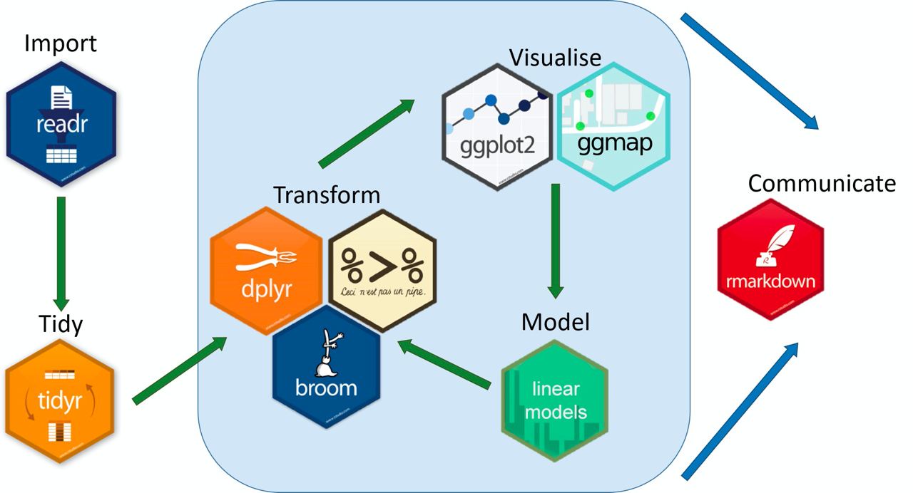
In this context of functional programming, a decade ago {tidyverse} was born, a “universe” of packages to guarantee an efficient, coherent and lexicographically simple to understand workflow, based on the idea that our data is clean and tidy.
What is tidyverse?

{lubridate}: date management{rvest}: web scraping{tidymodels}: modeling/prediction
{tibble}: optimizing data.frame{tidyr}: data cleaning{readr}: load rectangular data (.csv),{readxl}: import .xls and .xlsx files{dplyr}: grammar for debugging{stringr}: text handling{purrr}: list handling{forcats}: qualitative handling{ggplot2}: data visualization
What is tidyverse?

{lubridate}: date management{rvest}: web scraping{tidymodels}: modeling/prediction
{tibble}: optimizing data.frame{tidyr}: data cleaning{readr}: load rectangular data (.csv),{readxl}: import .xls and .xlsx files{dplyr}: grammar for debugging{stringr}: text handling{purrr}: list handling{forcats}: qualitative handling{ggplot2}: data visualization
Basic idea: tidy data
Tidy datasets are all alike, but every messy dataset is messy in its own way (Hadley Wickham, Chief Scientist en RStudio)
TIDYVERSE
The universe of {tidyverse} packages is based on the idea introduced by Hadley Wickham (the God we pray to) of standardizing the format of data to
- systematize debugging
- make it easier simpler to manipulate
- legible code.
Rules
The first thing will therefore be to understand what the tidydata sets are, since the whole {tidyverse} is based on the data being standardized.
- Each variable in a single column
- Each individual in a different row
- Each cell with a single value
- Each dataset in a tibble
- If we want to join multiple datasets we must have a common (key) column.

Pipe
In {tidyverse} the operator pipe (pipe) defined as |> (ctrl+shift+M) will be key: it will be a pipe that traverses the data and transforms it. . . .
In R base, if we want to apply three functions first(), second() and third() in order, it would be
Important
Since version 4.1.0 of R we have |>, a native pipe available outside tidyverse, replacing the old pipe %>% which depended on the {magrittr} package (quite problematic).
Pipe
The main advantage is that the code is very readable (almost literal) and you can do large operations on the data with very little code.
Messy data
But what does the non-tidy (messy) data look like? Let’s load the table4a table from the {tidyr} package (we already have it loaded from the {tidyverse} environment).
# A tibble: 3 × 3
  country     `1999` `2000`
  <chr>        <dbl>  <dbl>
1 Afghanistan    745   2666
2 Brazil       37737  80488
3 China       212258 213766
What could be wrong?
Pivot longer
❎ Each row represents two observations (1999 and 2000) → the columns 1999 and 2000 should actually themselves be values of a variable and not column names.
We will include a new column that stores the year and another one that stores the value of the variable of interest in each of those years. And we will do it with the pivot_longer() function: pivot the table to long format:
Pivot longer
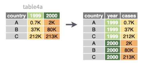
cols: name of the variables to pivot.names_to: name of the new variable to which we send the header of the table (the names).values_to: name of the new variable to which we are going to send the data.
Messy data
Let’s see another example with table table2.
# A tibble: 12 × 4
   country      year type            count
   <chr>       <dbl> <chr>           <dbl>
 1 Afghanistan  1999 cases             745
 2 Afghanistan  1999 population   19987071
 3 Afghanistan  2000 cases            2666
 4 Afghanistan  2000 population   20595360
 5 Brazil       1999 cases           37737
 6 Brazil       1999 population  172006362
 7 Brazil       2000 cases           80488
 8 Brazil       2000 population  174504898
 9 China        1999 cases          212258
10 China        1999 population 1272915272
11 China        2000 cases          213766
12 China        2000 population 1280428583
What could be wrong?
Pivot wider
# A tibble: 12 × 4
   country      year type            count
   <chr>       <dbl> <chr>           <dbl>
 1 Afghanistan  1999 cases             745
 2 Afghanistan  1999 population   19987071
 3 Afghanistan  2000 cases            2666
 4 Afghanistan  2000 population   20595360
 5 Brazil       1999 cases           37737
 6 Brazil       1999 population  172006362
 7 Brazil       2000 cases           80488
 8 Brazil       2000 population  174504898
 9 China        1999 cases          212258
10 China        1999 population 1272915272
11 China        2000 cases          213766
12 China        2000 population 1280428583
❎ Each observation is divided into two rows → the records with the same year should be the same
What we will do will be the opposite: with pivot_wider() we will widen the table
# A tibble: 6 × 4
  country      year  cases population
  <chr>       <dbl>  <dbl>      <dbl>
1 Afghanistan  1999    745   19987071
2 Afghanistan  2000   2666   20595360
3 Brazil       1999  37737  172006362
4 Brazil       2000  80488  174504898
5 China        1999 212258 1272915272
6 China        2000 213766 1280428583
Messy data
Let’s see another example with table table3.
# A tibble: 6 × 3
  country      year rate
  <chr>       <dbl> <chr>
1 Afghanistan  1999 745/19987071
2 Afghanistan  2000 2666/20595360
3 Brazil       1999 37737/172006362
4 Brazil       2000 80488/174504898
5 China        1999 212258/1272915272
6 China        2000 213766/1280428583
What could be wrong?
Separate
❎ Each cell contains several values
What we will do is make use of the separate() function to send separate each value to a different column.
# A tibble: 6 × 4
  country      year cases  pop
  <chr>       <dbl> <chr>  <chr>
1 Afghanistan  1999 745    19987071
2 Afghanistan  2000 2666   20595360
3 Brazil       1999 37737  172006362
4 Brazil       2000 80488  174504898
5 China        1999 212258 1272915272
6 China        2000 213766 1280428583
Separate
# A tibble: 6 × 4
  country      year cases  pop
  <chr>       <dbl> <chr>  <chr>
1 Afghanistan  1999 745    19987071
2 Afghanistan  2000 2666   20595360
3 Brazil       1999 37737  172006362
4 Brazil       2000 80488  174504898
5 China        1999 212258 1272915272
6 China        2000 213766 1280428583
Notice that the data, although it has separated them, kept them as text when in fact they should be numeric variables. For this we can add the optional argument convert = TRUE.
# A tibble: 6 × 4
  country      year  cases        pop
  <chr>       <dbl>  <int>      <int>
1 Afghanistan  1999    745   19987071
2 Afghanistan  2000   2666   20595360
3 Brazil       1999  37737  172006362
4 Brazil       2000  80488  174504898
5 China        1999 212258 1272915272
6 China        2000 213766 1280428583
Messy data
Let’s see the last example with table table5.
# A tibble: 6 × 4
  country     century year  rate
  <chr>       <chr>   <chr> <chr>
1 Afghanistan 19      99    745/19987071
2 Afghanistan 20      00    2666/20595360
3 Brazil      19      99    37737/172006362
4 Brazil      20      00    80488/174504898
5 China       19      99    212258/1272915272
6 China       20      00    213766/1280428583
What could be wrong?
Unite
❎ We have same values divided in two columns
We will use unite() to unite the values of century and year in the same column
# A tibble: 6 × 3
  country     whole_year rate
  <chr>       <chr>      <chr>
1 Afghanistan 1999       745/19987071
2 Afghanistan 2000       2666/20595360
3 Brazil      1999       37737/172006362
4 Brazil      2000       80488/174504898
5 China       1999       212258/1272915272
6 China       2000       213766/1280428583
Nest data
We can also nest datasets inside another one: imagine we have a dataset with variables x and y, with two records, another with one and another with 3 of them.
data <-
  tibble("dataset" = c(1, 1, 2, 3, 3, 3),
         "x" = c(0, 2, NA, -2, 6, 7),
         "y" = c(-1, NA, 5, 1.5, NA, -2))
data
# A tibble: 6 × 3
dataset x y
<dbl> <dbl> <dbl>
1 1 0 -1
2 1 2 NA
3 2 NA 5
4 3 -2 1.5
5 3 6 NA
6 3 7 -2 In reality everything that has an equal value in dataset should form its own tibble so let’s create one inside the one we have
Nest data
For it we will use the function nest() indicating it which variables form the datasets that will be nested (in this case variables x and y). Notice that inside what it stores is a variable of type list (since each dataset has a different length).
Nest data
To unnest just use the unnest() function indicating the column to unnest.
Example: world bank pop
In the {tidyr} package we have the world_bank_pop dataset which contains data from the World Bank about population per country from 2000 to 2018.
# A tibble: 1,064 × 20
   country indicator      `2000`  `2001`  `2002`  `2003`  `2004`  `2005`  `2006`
   <chr>   <chr>           <dbl>   <dbl>   <dbl>   <dbl>   <dbl>   <dbl>   <dbl>
 1 ABW     SP.URB.TOTL    4.16e4 4.20e+4 4.22e+4 4.23e+4 4.23e+4 4.24e+4 4.26e+4
 2 ABW     SP.URB.GROW    1.66e0 9.56e-1 4.01e-1 1.97e-1 9.46e-2 1.94e-1 3.67e-1
 3 ABW     SP.POP.TOTL    8.91e4 9.07e+4 9.18e+4 9.27e+4 9.35e+4 9.45e+4 9.56e+4
 4 ABW     SP.POP.GROW    2.54e0 1.77e+0 1.19e+0 9.97e-1 9.01e-1 1.00e+0 1.18e+0
 5 AFE     SP.URB.TOTL    1.16e8 1.20e+8 1.24e+8 1.29e+8 1.34e+8 1.39e+8 1.44e+8
 6 AFE     SP.URB.GROW    3.60e0 3.66e+0 3.72e+0 3.71e+0 3.74e+0 3.81e+0 3.81e+0
 7 AFE     SP.POP.TOTL    4.02e8 4.12e+8 4.23e+8 4.34e+8 4.45e+8 4.57e+8 4.70e+8
 8 AFE     SP.POP.GROW    2.58e0 2.59e+0 2.61e+0 2.62e+0 2.64e+0 2.67e+0 2.70e+0
 9 AFG     SP.URB.TOTL    4.31e6 4.36e+6 4.67e+6 5.06e+6 5.30e+6 5.54e+6 5.83e+6
10 AFG     SP.URB.GROW    1.86e0 1.15e+0 6.86e+0 7.95e+0 4.59e+0 4.47e+0 5.03e+0
# ℹ 1,054 more rows
# ℹ 11 more variables: `2007` <dbl>, `2008` <dbl>, `2009` <dbl>, `2010` <dbl>,
#   `2011` <dbl>, `2012` <dbl>, `2013` <dbl>, `2014` <dbl>, `2015` <dbl>,
#   `2016` <dbl>, `2017` <dbl>
What could be wrong?
Example: world bank pop
First of all, we can see that we effectively have the same variable in 18 columns: population.
What we should have is a column called pop with these values and another year indicating to which year corresponds the measurement. And for this we will do it with pivot_longer().
world_bank_pop_tidy <-
  world_bank_pop |>
  pivot_longer(cols = -(country:indicator), names_to = "year", values_to = "value")
world_bank_pop_tidy
# A tibble: 19,152 × 4
country indicator year value
<chr> <chr> <chr> <dbl>
1 ABW SP.URB.TOTL 2000 41625
2 ABW SP.URB.TOTL 2001 42025
3 ABW SP.URB.TOTL 2002 42194
4 ABW SP.URB.TOTL 2003 42277
5 ABW SP.URB.TOTL 2004 42317
6 ABW SP.URB.TOTL 2005 42399
7 ABW SP.URB.TOTL 2006 42555
8 ABW SP.URB.TOTL 2007 42729
9 ABW SP.URB.TOTL 2008 42906
10 ABW SP.URB.TOTL 2009 43079
# ℹ 19,142 more rowsExample: world bank pop
# A tibble: 19,152 × 4
   country indicator   year  value
   <chr>   <chr>       <chr> <dbl>
 1 ABW     SP.URB.TOTL 2000  41625
 2 ABW     SP.URB.TOTL 2001  42025
 3 ABW     SP.URB.TOTL 2002  42194
 4 ABW     SP.URB.TOTL 2003  42277
 5 ABW     SP.URB.TOTL 2004  42317
 6 ABW     SP.URB.TOTL 2005  42399
 7 ABW     SP.URB.TOTL 2006  42555
 8 ABW     SP.URB.TOTL 2007  42729
 9 ABW     SP.URB.TOTL 2008  42906
10 ABW     SP.URB.TOTL 2009  43079
# ℹ 19,142 more rowsIs everything correct?
Example: world bank pop
What should be done?
We will separate this variable into 3: one for the prefix SP (which we will eliminate later), one for the area (POP/URB) and one for the value (variable), which can be total or growth.
world_bank_pop_tidy2 <-
  world_bank_pop_tidy |>
  separate(indicator, c("dummy", "area", "variable"))
world_bank_pop_tidy2$dummy <- NULL
world_bank_pop_tidy2
# A tibble: 19,152 × 5
country area variable year value
<chr> <chr> <chr> <chr> <dbl>
1 ABW URB TOTL 2000 41625
2 ABW URB TOTL 2001 42025
3 ABW URB TOTL 2002 42194
4 ABW URB TOTL 2003 42277
5 ABW URB TOTL 2004 42317
6 ABW URB TOTL 2005 42399
7 ABW URB TOTL 2006 42555
8 ABW URB TOTL 2007 42729
9 ABW URB TOTL 2008 42906
10 ABW URB TOTL 2009 43079
# ℹ 19,142 more rowsExample: world bank pop
This can be done in a simpler way by indicating in the variable that we want to eliminate that it is NA inside separate().
world_bank_pop_tidy <-
  world_bank_pop_tidy |>
  separate(indicator, c(NA, "area", "variable"))
world_bank_pop_tidy
# A tibble: 19,152 × 5
country area variable year value
<chr> <chr> <chr> <chr> <dbl>
1 ABW URB TOTL 2000 41625
2 ABW URB TOTL 2001 42025
3 ABW URB TOTL 2002 42194
4 ABW URB TOTL 2003 42277
5 ABW URB TOTL 2004 42317
6 ABW URB TOTL 2005 42399
7 ABW URB TOTL 2006 42555
8 ABW URB TOTL 2007 42729
9 ABW URB TOTL 2008 42906
10 ABW URB TOTL 2009 43079
# ℹ 19,142 more rowsHave we got it yet? Think carefully: does each variable have its own column?
Example: world bank pop
If you actually look at the total population and growth variables, they should be different variables, since they even have different units: one is inhabitants, the other is percentage points.
To do the reverse of the initial operation, pivot_wider() (later we will use a tremendously useful function, {janitor}’s clean_names() which unifies variable names).
world_bank_pop_tidy <-
  world_bank_pop_tidy |>
  pivot_wider(names_from = "variable", values_from = "value") |>
  janitor::clean_names()
world_bank_pop_tidy
# A tibble: 9,576 × 5
country area year totl grow
<chr> <chr> <chr> <dbl> <dbl>
1 ABW URB 2000 41625 1.66
2 ABW URB 2001 42025 0.956
3 ABW URB 2002 42194 0.401
4 ABW URB 2003 42277 0.197
5 ABW URB 2004 42317 0.0946
6 ABW URB 2005 42399 0.194
7 ABW URB 2006 42555 0.367
8 ABW URB 2007 42729 0.408
9 ABW URB 2008 42906 0.413
10 ABW URB 2009 43079 0.402
# ℹ 9,566 more rowsExample: world bank pop
The complete code would be this: short, concise, readable and self-descriptive.
world_bank_pop_tidy <-
  world_bank_pop |>
  pivot_longer(cols = -(country:indicator), names_to = "year", values_to = "value") |>
  separate(indicator, c(NA, "area", "variable")) |>
  pivot_wider(names_from = "variable", values_from = "value") |>
  janitor::clean_names()
world_bank_pop_tidy
# A tibble: 9,576 × 5
country area year totl grow
<chr> <chr> <chr> <dbl> <dbl>
1 ABW URB 2000 41625 1.66
2 ABW URB 2001 42025 0.956
3 ABW URB 2002 42194 0.401
4 ABW URB 2003 42277 0.197
5 ABW URB 2004 42317 0.0946
6 ABW URB 2005 42399 0.194
7 ABW URB 2006 42555 0.367
8 ABW URB 2007 42729 0.408
9 ABW URB 2008 42906 0.413
10 ABW URB 2009 43079 0.402
# ℹ 9,566 more rowsExample: who dataset
In{tidyr} package we have who2 dataset (World Health Organization dataset)
# A tibble: 7,240 × 58
   country      year sp_m_014 sp_m_1524 sp_m_2534 sp_m_3544 sp_m_4554 sp_m_5564
   <chr>       <dbl>    <dbl>     <dbl>     <dbl>     <dbl>     <dbl>     <dbl>
 1 Afghanistan  1980       NA        NA        NA        NA        NA        NA
 2 Afghanistan  1981       NA        NA        NA        NA        NA        NA
 3 Afghanistan  1982       NA        NA        NA        NA        NA        NA
 4 Afghanistan  1983       NA        NA        NA        NA        NA        NA
 5 Afghanistan  1984       NA        NA        NA        NA        NA        NA
 6 Afghanistan  1985       NA        NA        NA        NA        NA        NA
 7 Afghanistan  1986       NA        NA        NA        NA        NA        NA
 8 Afghanistan  1987       NA        NA        NA        NA        NA        NA
 9 Afghanistan  1988       NA        NA        NA        NA        NA        NA
10 Afghanistan  1989       NA        NA        NA        NA        NA        NA
# ℹ 7,230 more rows
# ℹ 50 more variables: sp_m_65 <dbl>, sp_f_014 <dbl>, sp_f_1524 <dbl>,
#   sp_f_2534 <dbl>, sp_f_3544 <dbl>, sp_f_4554 <dbl>, sp_f_5564 <dbl>,
#   sp_f_65 <dbl>, sn_m_014 <dbl>, sn_m_1524 <dbl>, sn_m_2534 <dbl>,
#   sn_m_3544 <dbl>, sn_m_4554 <dbl>, sn_m_5564 <dbl>, sn_m_65 <dbl>,
#   sn_f_014 <dbl>, sn_f_1524 <dbl>, sn_f_2534 <dbl>, sn_f_3544 <dbl>,
#   sn_f_4554 <dbl>, sn_f_5564 <dbl>, sn_f_65 <dbl>, ep_m_014 <dbl>, …
Is it tidy data? Why?
Example: who dataset
First step for tidy data: we must pivot the table (tip: use paper and pen to sketch how the database should look like) so that there is a column called cases (since all columns starting from year is actually the same, cases of a disease).
who_tidy <-
  who2 |>
  pivot_longer(cols = -(country:year), names_to = "type", values_to = "cases")
who_tidy
# A tibble: 405,440 × 4
country year type cases
<chr> <dbl> <chr> <dbl>
1 Afghanistan 1980 sp_m_014 NA
2 Afghanistan 1980 sp_m_1524 NA
3 Afghanistan 1980 sp_m_2534 NA
4 Afghanistan 1980 sp_m_3544 NA
5 Afghanistan 1980 sp_m_4554 NA
6 Afghanistan 1980 sp_m_5564 NA
7 Afghanistan 1980 sp_m_65 NA
8 Afghanistan 1980 sp_f_014 NA
9 Afghanistan 1980 sp_f_1524 NA
10 Afghanistan 1980 sp_f_2534 NA
# ℹ 405,430 more rowsExample: who dataset
If you notice there are a lot of rows that do not make sense to keep because we have no cases! Investigate the pivot_longer() options to see how we can directly remove them in the pivot.
who_tidy <-
  who2 |>
  pivot_longer(cols = -(country:year), names_to = "type", values_to = "cases",
               values_drop_na = TRUE)
who_tidy
# A tibble: 76,046 × 4
country year type cases
<chr> <dbl> <chr> <dbl>
1 Afghanistan 1997 sp_m_014 0
2 Afghanistan 1997 sp_m_1524 10
3 Afghanistan 1997 sp_m_2534 6
4 Afghanistan 1997 sp_m_3544 3
5 Afghanistan 1997 sp_m_4554 5
6 Afghanistan 1997 sp_m_5564 2
7 Afghanistan 1997 sp_m_65 0
8 Afghanistan 1997 sp_f_014 5
9 Afghanistan 1997 sp_f_1524 38
10 Afghanistan 1997 sp_f_2534 36
# ℹ 76,036 more rowsExample: who dataset
Now in type we have coded the information as diagnosis_sex_age. How to separate it in 3 columns? Investigate both separate() and pivot_longer() options.
# separate
who_tidy <-
  who_tidy |>
  separate(col = "type", into = c("diagnosis", "sex", "age"))

# pivot_longer
who_tidy <-
  who2 |>
  pivot_longer(cols = -(country:year), names_to = c("diagnosis", "sex", "age"),
               values_to = "cases", values_drop_na = TRUE,
               names_sep = "_")
who_tidy
# A tibble: 76,046 × 6
country year diagnosis sex age cases
<chr> <dbl> <chr> <chr> <chr> <dbl>
1 Afghanistan 1997 sp m 014 0
2 Afghanistan 1997 sp m 1524 10
3 Afghanistan 1997 sp m 2534 6
4 Afghanistan 1997 sp m 3544 3
5 Afghanistan 1997 sp m 4554 5
6 Afghanistan 1997 sp m 5564 2
7 Afghanistan 1997 sp m 65 0
8 Afghanistan 1997 sp f 014 5
9 Afghanistan 1997 sp f 1524 38
10 Afghanistan 1997 sp f 2534 36
# ℹ 76,036 more rowsExample: who dataset
Finally, separate in two (age_inf, age_sup) the age range (which are numbers). Think about how to do it since it is not always 4 numbers (if there is no upper age range defined, put Inf as an upper bound).
who_tidy <-
  who_tidy |>
  separate(col = "age", into = c("age_inf", "age_sup"), sep = -2, convert = TRUE)
who_tidy$age_inf <- if_else(is.na(who_tidy$age_inf), 65, who_tidy$age_inf)
who_tidy$age_sup <- if_else(who_tidy$age_sup == 65, Inf, who_tidy$age_sup)
who_tidy
# A tibble: 76,046 × 7
country year diagnosis sex age_inf age_sup cases
<chr> <dbl> <chr> <chr> <dbl> <dbl> <dbl>
1 Afghanistan 1997 sp m 0 14 0
2 Afghanistan 1997 sp m 15 24 10
3 Afghanistan 1997 sp m 25 34 6
4 Afghanistan 1997 sp m 35 44 3
5 Afghanistan 1997 sp m 45 54 5
6 Afghanistan 1997 sp m 55 64 2
7 Afghanistan 1997 sp m 65 Inf 0
8 Afghanistan 1997 sp f 0 14 5
9 Afghanistan 1997 sp f 15 24 38
10 Afghanistan 1997 sp f 25 34 36
# ℹ 76,036 more rows💻 It’s your turn
Try to perform the following exercises without looking at the solutions
📝 Use the original who2 dataset from the {tidyr} package and try to answer the question: how many cases of tuberculosis were there in Spain in 1995 among women? Do it without converting it to tidydata. After that, pivot in a simple way and compare the code to be done when we have tidydata to when we don’t. Which one is more readable if you didn’t know R? Which one has higher error probability?
Código
# messy data
sum(who2[who2$country == "Spain" & who2$year == 1995,
     names(who2)[str_detect(names(who2), "f_")]], na.rm = TRUE)

# tidy data (at this moment)
sum(who_tidy[who_tidy$country == "Spain" &
           who_tidy$year == 1995 &
           who_tidy$sex == "f", ]$cases)

# in the future
who_tidy |>
  filter(country == "Spain" & year == 1995 & sex == "f") |>
  summarise(sum(cases))
📝 Using who_tidy determine which sex has had more cases, men or women? Create a new variable avg_age (mean age of the interval): if the range is 25 to 34, the mean age will be \((25 + 34)/2 = 29.5\) (if Inf above, NA)
📝 If we must choose a country in which we have the lowest probability of infection, which country, between the United Kingdom (United Kingdom of Great Britain and Northern Ireland) and France (similar population), had the fewest cases in the most recent year (whichever it was, even if the table was updated)?
📝 Take a look at table table4b in package {tidyr}. Is it tidydata? If not, what is wrong, how to convert it to tidy data in case it is not already?
🐣 Case study
Let’s perform a case study with the relig_income table in {tidyr} package. As indicated (? relig_income), the table represents the number of people in each annual income bracket (20k = 20 000$) and in each religion.
Try to answer the questions posed in the workbook
L2: tidyverse (rows)
Tidyverse: actions by rows
Preprocessing: dplyr
Within {tidyverse} we will use the {dplyr} package for the preprocessing process of the data.
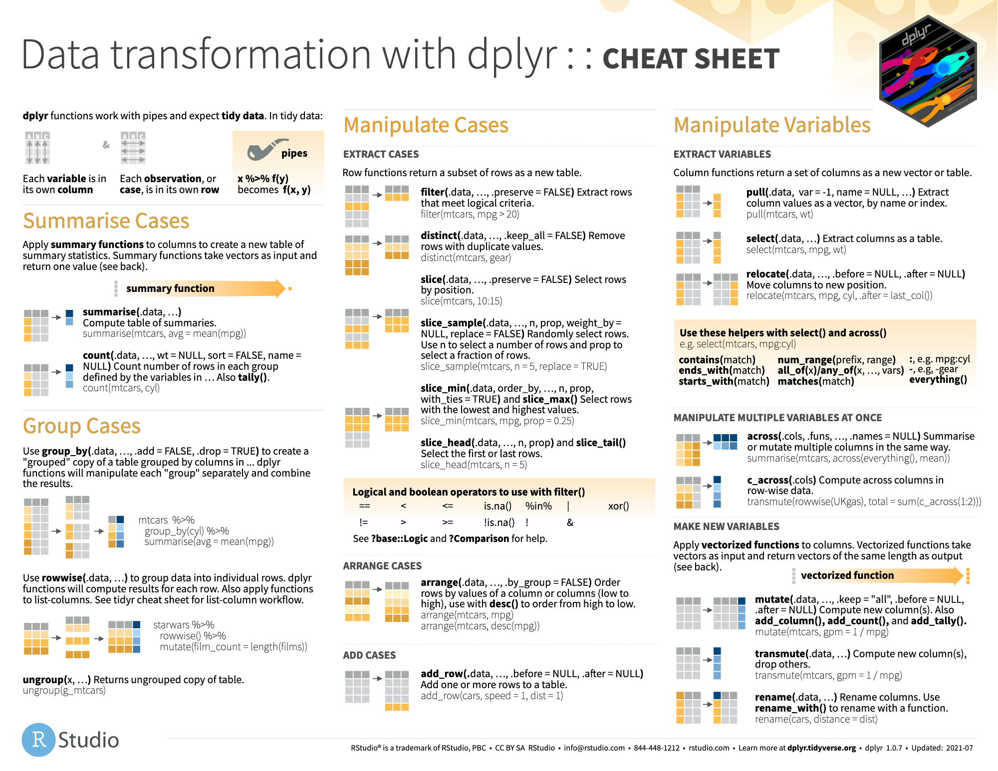
The idea is that the code is as readable as possible, as if it were a list of instructions that when read tells us in a very obvious way what it is doing.
Assumption: tidydata
All the preprocessing process we are going to perform is on the assumption that our data is in tidydata

Remember that in {tidyverse} the pipe operator defined as |> (ctrl+shift+M) will be key: it will be a pipe that traverses the data and transforms it.
Sampling
One of the most common operations is what is known in statistics as sampling: a selection or filtering of records (rows) (a subsample).
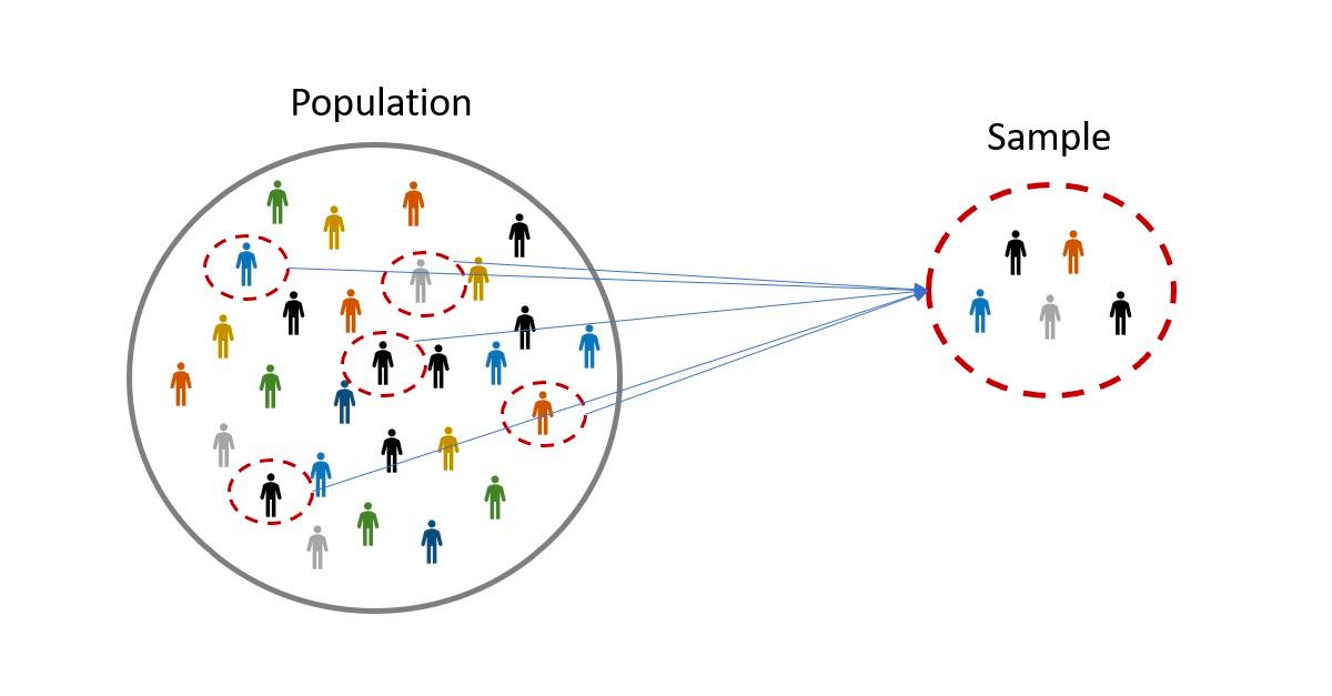
- Non-random (by quota): based on logical conditions on the records (
filter()).
- Non-random (intentional/discretionary): based on a position (
slice()).
- Simple random (
slice_sample()).
- Stratified (
group_by()+slice_sample()).
Filter rows: filter()
The simplest action by rows is when filter records based on some logical condition: with filter() only individuals meeting certain conditions will be selected (non-random sampling by conditions).
==,!=: equal or different to (|> filter(variable == "a"))>,<: greater or less than (|> filter(variable < 3))>=,<=: greater or equal or less or equal than (|> filter(variable >= 5))%in%: values belong to a set of discrete options (|> filter(variable %in% c("blue", "green")))between(variable, val1, val2): if continuous values are inside of a range (|> filter(between(variable, 160, 180)))
Filter rows: filter()
These logical conditions can be combined in different ways (and, or, or mutually exclusive).

Important
Remember that inside filter() there must always be something that returns a vector of logical values.
Filter rows: filter()
How would you go about… filter the characters with brown eyes?
What type of variable is it? –> The eye_color variable is qualitative so it is represented by texts.
# A tibble: 21 × 14
name height mass hair_color skin_color eye_color birth_year sex gender
<chr> <int> <dbl> <chr> <chr> <chr> <dbl> <chr> <chr>
1 Leia Or… 150 49 brown light brown 19 fema… femin…
2 Biggs D… 183 84 black light brown 24 male mascu…
3 Han Solo 180 80 brown fair brown 29 male mascu…
4 Yoda 66 17 white green brown 896 male mascu…
5 Boba Fe… 183 78.2 black fair brown 31.5 male mascu…
6 Lando C… 177 79 black dark brown 31 male mascu…
7 Arvel C… NA NA brown fair brown NA male mascu…
8 Wicket … 88 20 brown brown brown 8 male mascu…
9 Padmé A… 185 45 brown light brown 46 fema… femin…
10 Quarsh … 183 NA black dark brown 62 male mascu…
# ℹ 11 more rows
# ℹ 5 more variables: homeworld <chr>, species <chr>, films <list>,
# vehicles <list>, starships <list>Filter rows: filter()
How would you go about… filter the characters that do not have brown eyes?
# A tibble: 66 × 14
name height mass hair_color skin_color eye_color birth_year sex gender
<chr> <int> <dbl> <chr> <chr> <chr> <dbl> <chr> <chr>
1 Luke Sk… 172 77 blond fair blue 19 male mascu…
2 C-3PO 167 75 <NA> gold yellow 112 none mascu…
3 R2-D2 96 32 <NA> white, bl… red 33 none mascu…
4 Darth V… 202 136 none white yellow 41.9 male mascu…
5 Owen La… 178 120 brown, gr… light blue 52 male mascu…
6 Beru Wh… 165 75 brown light blue 47 fema… femin…
7 R5-D4 97 32 <NA> white, red red NA none mascu…
8 Obi-Wan… 182 77 auburn, w… fair blue-gray 57 male mascu…
9 Anakin … 188 84 blond fair blue 41.9 male mascu…
10 Wilhuff… 180 NA auburn, g… fair blue 64 male mascu…
# ℹ 56 more rows
# ℹ 5 more variables: homeworld <chr>, species <chr>, films <list>,
# vehicles <list>, starships <list>Filter rows: filter()
How would you go about … filter characters that have brown or blue eyes?
# A tibble: 40 × 14
name height mass hair_color skin_color eye_color birth_year sex gender
<chr> <int> <dbl> <chr> <chr> <chr> <dbl> <chr> <chr>
1 Luke Sk… 172 77 blond fair blue 19 male mascu…
2 Leia Or… 150 49 brown light brown 19 fema… femin…
3 Owen La… 178 120 brown, gr… light blue 52 male mascu…
4 Beru Wh… 165 75 brown light blue 47 fema… femin…
5 Biggs D… 183 84 black light brown 24 male mascu…
6 Anakin … 188 84 blond fair blue 41.9 male mascu…
7 Wilhuff… 180 NA auburn, g… fair blue 64 male mascu…
8 Chewbac… 228 112 brown unknown blue 200 male mascu…
9 Han Solo 180 80 brown fair brown 29 male mascu…
10 Jek Ton… 180 110 brown fair blue NA <NA> <NA>
# ℹ 30 more rows
# ℹ 5 more variables: homeworld <chr>, species <chr>, films <list>,
# vehicles <list>, starships <list>Filter rows: filter()
Note that %in% is equivalent to concatenating several == with a conjunction or (|)
# A tibble: 40 × 14
name height mass hair_color skin_color eye_color birth_year sex gender
<chr> <int> <dbl> <chr> <chr> <chr> <dbl> <chr> <chr>
1 Luke Sk… 172 77 blond fair blue 19 male mascu…
2 Leia Or… 150 49 brown light brown 19 fema… femin…
3 Owen La… 178 120 brown, gr… light blue 52 male mascu…
4 Beru Wh… 165 75 brown light blue 47 fema… femin…
5 Biggs D… 183 84 black light brown 24 male mascu…
6 Anakin … 188 84 blond fair blue 41.9 male mascu…
7 Wilhuff… 180 NA auburn, g… fair blue 64 male mascu…
8 Chewbac… 228 112 brown unknown blue 200 male mascu…
9 Han Solo 180 80 brown fair brown 29 male mascu…
10 Jek Ton… 180 110 brown fair blue NA <NA> <NA>
# ℹ 30 more rows
# ℹ 5 more variables: homeworld <chr>, species <chr>, films <list>,
# vehicles <list>, starships <list>Filter rows: filter()
How would you go about … filter the characters that are between 120 and 160 cm?
What type of variable is it? –> The variable height is a continuous quantitative variable so we must filter by ranges of values (intervals) –> we will use between().
# A tibble: 6 × 14
name height mass hair_color skin_color eye_color birth_year sex gender
<chr> <int> <dbl> <chr> <chr> <chr> <dbl> <chr> <chr>
1 Leia Org… 150 49 brown light brown 19 fema… femin…
2 Mon Moth… 150 NA auburn fair blue 48 fema… femin…
3 Nien Nunb 160 68 none grey black NA male mascu…
4 Watto 137 NA black blue, grey yellow NA male mascu…
5 Gasgano 122 NA none white, bl… black NA male mascu…
6 Cordé 157 NA brown light brown NA <NA> <NA>
# ℹ 5 more variables: homeworld <chr>, species <chr>, films <list>,
# vehicles <list>, starships <list>Filter rows: filter()
How would you… filter characters that have eyes and are not human?
# A tibble: 3 × 14
name height mass hair_color skin_color eye_color birth_year sex gender
<chr> <int> <dbl> <chr> <chr> <chr> <dbl> <chr> <chr>
1 Yoda 66 17 white green brown 896 male mascu…
2 Wicket S… 88 20 brown brown brown 8 male mascu…
3 Eeth Koth 171 NA black brown brown NA male mascu…
# ℹ 5 more variables: homeworld <chr>, species <chr>, films <list>,
# vehicles <list>, starships <list>Filter rows: filter()
How would you… filter characters that have eyes and are not human, or are over 60 years old? Think it through: the parentheses are important: \((a+b)*c\) is not the same as \(a+(b*c)\).
# A tibble: 18 × 14
name height mass hair_color skin_color eye_color birth_year sex gender
<chr> <int> <dbl> <chr> <chr> <chr> <dbl> <chr> <chr>
1 C-3PO 167 75 <NA> gold yellow 112 none mascu…
2 Wilhuff… 180 NA auburn, g… fair blue 64 male mascu…
3 Chewbac… 228 112 brown unknown blue 200 male mascu…
4 Jabba D… 175 1358 <NA> green-tan… orange 600 herm… mascu…
5 Yoda 66 17 white green brown 896 male mascu…
6 Palpati… 170 75 grey pale yellow 82 male mascu…
7 Wicket … 88 20 brown brown brown 8 male mascu…
8 Qui-Gon… 193 89 brown fair blue 92 male mascu…
9 Finis V… 170 NA blond fair blue 91 male mascu…
10 Quarsh … 183 NA black dark brown 62 male mascu…
11 Shmi Sk… 163 NA black fair brown 72 fema… femin…
12 Mace Wi… 188 84 none dark brown 72 male mascu…
13 Ki-Adi-… 198 82 white pale yellow 92 male mascu…
14 Eeth Ko… 171 NA black brown brown NA male mascu…
15 Cliegg … 183 NA brown fair blue 82 male mascu…
16 Dooku 193 80 white fair brown 102 male mascu…
17 Bail Pr… 191 NA black tan brown 67 male mascu…
18 Jango F… 183 79 black tan brown 66 male mascu…
# ℹ 5 more variables: homeworld <chr>, species <chr>, films <list>,
# vehicles <list>, starships <list>Drop missings: drop_na()
There is a special filter for one of the most common operations in debugging: remove absent. For this we can use inside a filter is.na(), which returns TRUE/FALSE depending on whether it is absent, or …
Use drop_na(): if we do not specify a variable, it removes records with missing in any variable. Later on we will see how to impute those missing
# A tibble: 7 × 4
name mass height hair_color
<chr> <dbl> <int> <chr>
1 Luke Skywalker 77 172 blond
2 C-3PO 75 167 <NA>
3 R2-D2 32 96 <NA>
4 Darth Vader 136 202 none
5 Leia Organa 49 150 brown
6 Owen Lars 120 178 brown, grey
7 Beru Whitesun Lars 75 165 brown # A tibble: 7 × 4
name mass height hair_color
<chr> <dbl> <int> <chr>
1 Luke Skywalker 77 172 blond
2 Darth Vader 136 202 none
3 Leia Organa 49 150 brown
4 Owen Lars 120 178 brown, grey
5 Beru Whitesun Lars 75 165 brown
6 Biggs Darklighter 84 183 black
7 Obi-Wan Kenobi 77 182 auburn, white💻 It’s your turn
Try to perform the following exercises without looking at the solutions
📝 Select from the starwars set only those characters that are androids or whose species value is unknown.
📝 Select from the starwars set only the characters whose weight is between 65 and 90 kg.
📝 After clearing absent in all variables, select from the starwars set only the characters that are human and come from Tatooine.
📝 Select from the original starwars set non-human characters, male in sex and measuring between 120 and 170 cm, or characters with brown or red eyes.
📝 Look for information in the str_detect() function help of the {stringr} package (loaded in {tidyverse}). Tip: test the functions you are going to use with some test vector beforehand so that you can check how they work. After you know what it does, filter out only those characters with the last name Skywalker.
Slices of data: slice()
Sometimes we may be interested in performing a non-random discretionary sampling, or in other words, filter by position: with slice(positions) we can select specific rows by passing as argument a index vector.
# A tibble: 1 × 4
name height mass hair_color
<chr> <int> <dbl> <chr>
1 Luke Skywalker 172 77 blond # A tibble: 4 × 8
name height mass hair_color skin_color eye_color birth_year sex
<chr> <int> <dbl> <chr> <chr> <chr> <dbl> <chr>
1 C-3PO 167 75 <NA> gold yellow 112 none
2 Beru Whitesun L… 165 75 brown light blue 47 fema…
3 Obi-Wan Kenobi 182 77 auburn, w… fair blue-gray 57 male
4 Qui-Gon Jinn 193 89 brown fair blue 92 male Slices of data: slice()
We have default options:
- with
slice_head(n = ...)andslice_tail(n = ...)we can get the header and tail of the table
Slices of data: slice()
We have default options:
- with
slice_max()andslice_min()we get the rows with smallest/largest value of a variable (if tie, all unlesswith_ties = FALSE) which we indicate inorder_by = ....
# A tibble: 2 × 4
name height mass hair_color
<chr> <int> <dbl> <chr>
1 Ratts Tyerel 79 15 none
2 Yoda 66 17 white Random sampling: slice_sample()
The so-called simple random sampling is based on selecting individuals randomly, so that each one has certain probabilities of being selected. With slice_sample(n = ...) we can randomly extract n (a priori equiprobable) records.
# A tibble: 2 × 14
name height mass hair_color skin_color eye_color birth_year sex gender
<chr> <int> <dbl> <chr> <chr> <chr> <dbl> <chr> <chr>
1 Dexter J… 198 102 none brown yellow NA male mascu…
2 Ratts Ty… 79 15 none grey, blue unknown NA male mascu…
# ℹ 5 more variables: homeworld <chr>, species <chr>, films <list>,
# vehicles <list>, starships <list>Important
“Random” does not imply equiprobable: a normal die is just as random as a trick die. There are no things “more random” than others, they simply have different underlying probability laws.
Random sampling: slice_sample()
We can also indicate the proportion of data to sample (instead of the number) and if we want it to be with replacement (that can be repeated).
# A tibble: 4 × 14
name height mass hair_color skin_color eye_color birth_year sex gender
<chr> <int> <dbl> <chr> <chr> <chr> <dbl> <chr> <chr>
1 Leia Org… 150 49 brown light brown 19 fema… femin…
2 Yoda 66 17 white green brown 896 male mascu…
3 Biggs Da… 183 84 black light brown 24 male mascu…
4 Darth Ma… 175 80 none red yellow 54 male mascu…
# ℹ 5 more variables: homeworld <chr>, species <chr>, films <list>,
# vehicles <list>, starships <list>Random sampling: slice_sample()
As we said, “random” is not the same as “equiprobable”, so we can pass a probability vector. For example, let’s force that it is very improbable to draw a row other than the first two rows
# A tibble: 2 × 14
name height mass hair_color skin_color eye_color birth_year sex gender
<chr> <int> <dbl> <chr> <chr> <chr> <dbl> <chr> <chr>
1 Luke Sky… 172 77 blond fair blue 19 male mascu…
2 C-3PO 167 75 <NA> gold yellow 112 none mascu…
# ℹ 5 more variables: homeworld <chr>, species <chr>, films <list>,
# vehicles <list>, starships <list># A tibble: 2 × 14
name height mass hair_color skin_color eye_color birth_year sex gender
<chr> <int> <dbl> <chr> <chr> <chr> <dbl> <chr> <chr>
1 C-3PO 167 75 <NA> gold yellow 112 none mascu…
2 Luke Sky… 172 77 blond fair blue 19 male mascu…
# ℹ 5 more variables: homeworld <chr>, species <chr>, films <list>,
# vehicles <list>, starships <list>sample()
The slice_sample() function is simply a {tidyverse} integration of the basic R function known as sample() that allows us to sample elements
sample()
The previous option generates events of a random variable equiprobable but as before, we can assign a vector of probabilities or mass function to it with the argument prob = ....
sample()
How would you make the following statement?
Suppose that seasonal flu episodes have been studied in a city. Let \(X_m\) and \(X_p\) be random variables such that \(X_m=1\) if the mother has flu, \(X_m=0\) if the mother does not have flu, \(X_p=1\) if the father has flu and \(X_p=0\) if the father does not have flu. The theoretical model associated with this type of epidemics indicates that the joint distribution is given by \(P(X_m = 1, X_p=1)=0.02\), \(P(X_m = 1, X_p=0)=0.08\), \(P(X_m = 1, X_p=0)=0. 1\) and \(P(X_m = 0, X_p=0)=0.8\)
Generate a sample of size \(n = 1000\) (support "10", "01", "00" and "11") by making use of runif() and by making use of sample().
Sort by rows: arrange()
We can also order by rows according to some variable with arrange().
# A tibble: 5 × 6
name height mass hair_color skin_color eye_color
<chr> <int> <dbl> <chr> <chr> <chr>
1 Ratts Tyerel 79 15 none grey, blue unknown
2 Yoda 66 17 white green brown
3 Wicket Systri Warrick 88 20 brown brown brown
4 R2-D2 96 32 <NA> white, blue red
5 R5-D4 97 32 <NA> white, red red By from lowest to highest but we can reverse the order with desc().
# A tibble: 5 × 3
name height mass
<chr> <int> <dbl>
1 Yarael Poof 264 NA
2 Tarfful 234 136
3 Lama Su 229 88
4 Chewbacca 228 112
5 Roos Tarpals 224 82Remove duplicates: distinct()
Many times we will need to make sure that there are no duplicates in some variable (DNI) and we can delete duplicate rows with distinct().
# A tibble: 5 × 1
sex
<chr>
1 male
2 none
3 female
4 hermaphroditic
5 <NA> To keep all the columns of the table we will use .keep_all = TRUE.
# A tibble: 3 × 14
name height mass hair_color skin_color eye_color birth_year sex gender
<chr> <int> <dbl> <chr> <chr> <chr> <dbl> <chr> <chr>
1 Luke Sky… 172 77 blond fair blue 19 male mascu…
2 C-3PO 167 75 <NA> gold yellow 112 none mascu…
3 Leia Org… 150 49 brown light brown 19 fema… femin…
# ℹ 5 more variables: homeworld <chr>, species <chr>, films <list>,
# vehicles <list>, starships <list>Including rows: bind_rows()
Finally, we can bind new rows with bind_rows() with new observations in table (if columns do not match fill with absent)
# A tibble: 2 × 2
name age
<chr> <dbl>
1 javi 33
2 laura 50💻 It’s your turn
Try to perform the following exercises without looking at the solutions
📝 Select only the characters that are human and brown-eyed, then sort them in descending height and ascending weight.
📝R andomly draws 10 characters but in such a way that the probability of each character being drawn is proportional to its weight (heavier, more likely).
📝 To find out what unique values are in the hair color, remove duplicates of the hair_color variable by first removing the missing ones from the hair_color variable.
📝 Of the characters that are human and taller than 160 cm, eliminate duplicates in eye color, eliminate absent in weight, select the 3 tallest, and order from tallest to shortest in weight. Return the table.
🐣 Case study
Let’s go back to a known dataset: in the {datasets} package (already installed by default) we had several datasets and one of them was airquality which we already worked with. The data captures daily measurements (n = 153 observations) of air quality in New York, from May to September 1973.
At that time we worked it from the R base perspective and extracted some variables from it. The objective now will be to work it from the {tidyverse} perspective looking at the differences from one form to the other.
Try to answer the questions posed in the workbook.
L3: tidyverse (columns)
Tidyverse: actions by columns
Select columns: select()
Up to now all operations performed (even if we used column info) were by rows. In the case of columns, the simplest action is to select variables by name with select(), giving as arguments the column names without quotes.
# A tibble: 87 × 2
name hair_color
<chr> <chr>
1 Luke Skywalker blond
2 C-3PO <NA>
3 R2-D2 <NA>
4 Darth Vader none
5 Leia Organa brown
6 Owen Lars brown, grey
7 Beru Whitesun Lars brown
8 R5-D4 <NA>
9 Biggs Darklighter black
10 Obi-Wan Kenobi auburn, white
# ℹ 77 more rowsSelect columns: select()
The select() function allows us to select several variables at once, including concatenating their names as if they were numerical indexes with :
# A tibble: 4 × 6
name height mass hair_color skin_color eye_color
<chr> <int> <dbl> <chr> <chr> <chr>
1 Luke Skywalker 172 77 blond fair blue
2 C-3PO 167 75 <NA> gold yellow
3 R2-D2 96 32 <NA> white, blue red
4 Darth Vader 202 136 none white yellow Select columns: select()
We have also reserved words: everything() all variables….
# A tibble: 4 × 14
mass homeworld name height hair_color skin_color eye_color birth_year sex
<dbl> <chr> <chr> <int> <chr> <chr> <chr> <dbl> <chr>
1 77 Tatooine Luke … 172 blond fair blue 19 male
2 75 Tatooine C-3PO 167 <NA> gold yellow 112 none
3 32 Naboo R2-D2 96 <NA> white, bl… red 33 none
4 136 Tatooine Darth… 202 none white yellow 41.9 male
# ℹ 5 more variables: gender <chr>, species <chr>, films <list>,
# vehicles <list>, starships <list>…and last_col() to refer to last column.
# A tibble: 4 × 5
name height mass homeworld starships
<chr> <int> <dbl> <chr> <list>
1 Luke Skywalker 172 77 Tatooine <chr [2]>
2 C-3PO 167 75 Tatooine <chr [0]>
3 R2-D2 96 32 Naboo <chr [0]>
4 Darth Vader 202 136 Tatooine <chr [1]>Select columns: select()
We can also play with patterns in the name, those that begin with a prefix (starts_with()), [end with a suffix]{. hl-purple} (ends_with()), contain text (contains()) or fulfill a regular expression (matches()).
# variables which col name finish as "color" and contains sex and gender
starwars |> select(ends_with("color"), matches("sex|gender"))# A tibble: 87 × 5
hair_color skin_color eye_color sex gender
<chr> <chr> <chr> <chr> <chr>
1 blond fair blue male masculine
2 <NA> gold yellow none masculine
3 <NA> white, blue red none masculine
4 none white yellow male masculine
5 brown light brown female feminine
6 brown, grey light blue male masculine
7 brown light blue female feminine
8 <NA> white, red red none masculine
9 black light brown male masculine
10 auburn, white fair blue-gray male masculine
# ℹ 77 more rowsSelect columns: select()
We can even select by numeric range if we have variables with a prefix and numbers.
Select columns: select()
Finally, we can select columns by datatatype using where() and inside a function that returns a logical value of datatype.
# A tibble: 87 × 11
height mass birth_year name hair_color skin_color eye_color sex gender
<int> <dbl> <dbl> <chr> <chr> <chr> <chr> <chr> <chr>
1 172 77 19 Luke Sk… blond fair blue male mascu…
2 167 75 112 C-3PO <NA> gold yellow none mascu…
3 96 32 33 R2-D2 <NA> white, bl… red none mascu…
4 202 136 41.9 Darth V… none white yellow male mascu…
5 150 49 19 Leia Or… brown light brown fema… femin…
6 178 120 52 Owen La… brown, gr… light blue male mascu…
7 165 75 47 Beru Wh… brown light blue fema… femin…
8 97 32 NA R5-D4 <NA> white, red red none mascu…
9 183 84 24 Biggs D… black light brown male mascu…
10 182 77 57 Obi-Wan… auburn, w… fair blue-gray male mascu…
# ℹ 77 more rows
# ℹ 2 more variables: homeworld <chr>, species <chr>Move columns: relocate()
To facilitate the relocation of variables we have a function for it, relocate(), indicating in .after or .before behind or in front of which columns we want to move them.
# A tibble: 87 × 14
species name height mass hair_color skin_color eye_color birth_year sex
<chr> <chr> <int> <dbl> <chr> <chr> <chr> <dbl> <chr>
1 Human Luke S… 172 77 blond fair blue 19 male
2 Droid C-3PO 167 75 <NA> gold yellow 112 none
3 Droid R2-D2 96 32 <NA> white, bl… red 33 none
4 Human Darth … 202 136 none white yellow 41.9 male
5 Human Leia O… 150 49 brown light brown 19 fema…
6 Human Owen L… 178 120 brown, gr… light blue 52 male
7 Human Beru W… 165 75 brown light blue 47 fema…
8 Droid R5-D4 97 32 <NA> white, red red NA none
9 Human Biggs … 183 84 black light brown 24 male
10 Human Obi-Wa… 182 77 auburn, w… fair blue-gray 57 male
# ℹ 77 more rows
# ℹ 5 more variables: gender <chr>, homeworld <chr>, films <list>,
# vehicles <list>, starships <list>Rename: rename()
Sometimes we may also want to modify the “meta-information” of the data, renaming columns. To do this we will use rename() by typing first the new name and then the old.
# A tibble: 87 × 14
nombre altura peso hair_color skin_color eye_color birth_year sex gender
<chr> <int> <dbl> <chr> <chr> <chr> <dbl> <chr> <chr>
1 Luke Sk… 172 77 blond fair blue 19 male mascu…
2 C-3PO 167 75 <NA> gold yellow 112 none mascu…
3 R2-D2 96 32 <NA> white, bl… red 33 none mascu…
4 Darth V… 202 136 none white yellow 41.9 male mascu…
5 Leia Or… 150 49 brown light brown 19 fema… femin…
6 Owen La… 178 120 brown, gr… light blue 52 male mascu…
7 Beru Wh… 165 75 brown light blue 47 fema… femin…
8 R5-D4 97 32 <NA> white, red red NA none mascu…
9 Biggs D… 183 84 black light brown 24 male mascu…
10 Obi-Wan… 182 77 auburn, w… fair blue-gray 57 male mascu…
# ℹ 77 more rows
# ℹ 5 more variables: homeworld <chr>, species <chr>, films <list>,
# vehicles <list>, starships <list>Extract columns: pull()
If you look at the output of the select() still a tibble table, it preserves the nature of our data.
Extract columns: pull()
Sometimes we will not want such a structure but literally extract the column in a VECTOR, something we can do with pull().
[1] "Luke Skywalker" "C-3PO" "R2-D2"
[4] "Darth Vader" "Leia Organa" "Owen Lars"
[7] "Beru Whitesun Lars" "R5-D4" "Biggs Darklighter"
[10] "Obi-Wan Kenobi" "Anakin Skywalker" "Wilhuff Tarkin"
[13] "Chewbacca" "Han Solo" "Greedo"
[16] "Jabba Desilijic Tiure" "Wedge Antilles" "Jek Tono Porkins"
[19] "Yoda" "Palpatine" "Boba Fett"
[22] "IG-88" "Bossk" "Lando Calrissian"
[25] "Lobot" "Ackbar" "Mon Mothma"
[28] "Arvel Crynyd" "Wicket Systri Warrick" "Nien Nunb"
[31] "Qui-Gon Jinn" "Nute Gunray" "Finis Valorum"
[34] "Padmé Amidala" "Jar Jar Binks" "Roos Tarpals"
[37] "Rugor Nass" "Ric Olié" "Watto"
[40] "Sebulba" "Quarsh Panaka" "Shmi Skywalker"
[43] "Darth Maul" "Bib Fortuna" "Ayla Secura"
[46] "Ratts Tyerel" "Dud Bolt" "Gasgano"
[49] "Ben Quadinaros" "Mace Windu" "Ki-Adi-Mundi"
[52] "Kit Fisto" "Eeth Koth" "Adi Gallia"
[55] "Saesee Tiin" "Yarael Poof" "Plo Koon"
[58] "Mas Amedda" "Gregar Typho" "Cordé"
[61] "Cliegg Lars" "Poggle the Lesser" "Luminara Unduli"
[64] "Barriss Offee" "Dormé" "Dooku"
[67] "Bail Prestor Organa" "Jango Fett" "Zam Wesell"
[70] "Dexter Jettster" "Lama Su" "Taun We"
[73] "Jocasta Nu" "R4-P17" "Wat Tambor"
[76] "San Hill" "Shaak Ti" "Grievous"
[79] "Tarfful" "Raymus Antilles" "Sly Moore"
[82] "Tion Medon" "Finn" "Rey"
[85] "Poe Dameron" "BB8" "Captain Phasma" 💻 It’s your turn
Try to perform the following exercises without looking at the solutions
📝 Filter the set of characters and keep only those that do not have a missing data in the height variable. With the data obtained from the previous filter, select only the variables name, height, as well as all those variables that CONTAIN the word color in their name.
📝 With the data obtained from the previous Exercise, translate the names of the columns into Spanish (or your motherlanguage).
📝 With the data obtained from Exercise 1, place the hair color variable just after the name variable.
Con los data obtenidos del Exercise anterior, coloca la variable de color de pelo justo detrás de la variable de nombres.
📝 With the data obtained from the Exercise 1, check how many unique modalities there are in the hair color variable (without using unique()).
📝 From the original data set, it removes the list type columns, and then removes duplicates in the eye_color variable. After removing duplicates it extracts that column into a vector.
📝 From the original starwars dataset, with only the characters whose height is known, extract in a vector with that variable.
📝 After obtaining the vector from the previous Exercise, use this vector to randomly sample 50% of the data so that the probability of each character being chosen is inversely proportional to their height (shorter, more options).
Modify columns: mutate()
In many occasions we will want to modify or create variables with mutate().
Let’s create for example a new variable height_m with the height in meters.
# A tibble: 87 × 15
name height mass hair_color skin_color eye_color birth_year sex gender
<chr> <int> <dbl> <chr> <chr> <chr> <dbl> <chr> <chr>
1 Luke Sk… 172 77 blond fair blue 19 male mascu…
2 C-3PO 167 75 <NA> gold yellow 112 none mascu…
3 R2-D2 96 32 <NA> white, bl… red 33 none mascu…
4 Darth V… 202 136 none white yellow 41.9 male mascu…
5 Leia Or… 150 49 brown light brown 19 fema… femin…
6 Owen La… 178 120 brown, gr… light blue 52 male mascu…
7 Beru Wh… 165 75 brown light blue 47 fema… femin…
8 R5-D4 97 32 <NA> white, red red NA none mascu…
9 Biggs D… 183 84 black light brown 24 male mascu…
10 Obi-Wan… 182 77 auburn, w… fair blue-gray 57 male mascu…
# ℹ 77 more rows
# ℹ 6 more variables: homeworld <chr>, species <chr>, films <list>,
# vehicles <list>, starships <list>, height_m <dbl>Modify columns: mutate()
In addition with the optional arguments we can reposition the modified column
# A tibble: 87 × 16
height_m BMI name height mass hair_color skin_color eye_color birth_year
<dbl> <dbl> <chr> <int> <dbl> <chr> <chr> <chr> <dbl>
1 1.72 26.0 Luke … 172 77 blond fair blue 19
2 1.67 26.9 C-3PO 167 75 <NA> gold yellow 112
3 0.96 34.7 R2-D2 96 32 <NA> white, bl… red 33
4 2.02 33.3 Darth… 202 136 none white yellow 41.9
5 1.5 21.8 Leia … 150 49 brown light brown 19
6 1.78 37.9 Owen … 178 120 brown, gr… light blue 52
7 1.65 27.5 Beru … 165 75 brown light blue 47
8 0.97 34.0 R5-D4 97 32 <NA> white, red red NA
9 1.83 25.1 Biggs… 183 84 black light brown 24
10 1.82 23.2 Obi-W… 182 77 auburn, w… fair blue-gray 57
# ℹ 77 more rows
# ℹ 7 more variables: sex <chr>, gender <chr>, homeworld <chr>, species <chr>,
# films <list>, vehicles <list>, starships <list>Modify columns: mutate()
Important
When we apply mutate(), we must remember that the operations are performed vector by vector, element by element, so the function we use inside must return a vector of equal length. Otherwise, it will return a constant.
# A tibble: 87 × 15
constante name height mass hair_color skin_color eye_color birth_year sex
<dbl> <chr> <int> <dbl> <chr> <chr> <chr> <dbl> <chr>
1 97.3 Luke… 172 77 blond fair blue 19 male
2 97.3 C-3PO 167 75 <NA> gold yellow 112 none
3 97.3 R2-D2 96 32 <NA> white, bl… red 33 none
4 97.3 Dart… 202 136 none white yellow 41.9 male
5 97.3 Leia… 150 49 brown light brown 19 fema…
6 97.3 Owen… 178 120 brown, gr… light blue 52 male
7 97.3 Beru… 165 75 brown light blue 47 fema…
8 97.3 R5-D4 97 32 <NA> white, red red NA none
9 97.3 Bigg… 183 84 black light brown 24 male
10 97.3 Obi-… 182 77 auburn, w… fair blue-gray 57 male
# ℹ 77 more rows
# ℹ 6 more variables: gender <chr>, homeworld <chr>, species <chr>,
# films <list>, vehicles <list>, starships <list>Recategorize: if_else()
We can also combine mutate() with the if_else() control expression to recategorize the variable: if a condition is met, it does one thing, otherwise another.
starwars |>
mutate(human = if_else(species == "Human", "Human", "Not Human"),
.after = name) |>
select(name:mass)# A tibble: 87 × 4
name human height mass
<chr> <chr> <int> <dbl>
1 Luke Skywalker Human 172 77
2 C-3PO Not Human 167 75
3 R2-D2 Not Human 96 32
4 Darth Vader Human 202 136
5 Leia Organa Human 150 49
6 Owen Lars Human 178 120
7 Beru Whitesun Lars Human 165 75
8 R5-D4 Not Human 97 32
9 Biggs Darklighter Human 183 84
10 Obi-Wan Kenobi Human 182 77
# ℹ 77 more rowsRecategorize: case_when()
For more complex categorizations we have case_when(), for example, to create a category of characters based on their height.
starwars |>
drop_na(height) |>
mutate(altura = case_when(height < 120 ~ "dwarf",
height < 160 ~ "short",
height < 180 ~ "normal",
height < 200 ~ "tall",
TRUE ~ "giant"), .before = name)# A tibble: 81 × 15
altura name height mass hair_color skin_color eye_color birth_year sex
<chr> <chr> <int> <dbl> <chr> <chr> <chr> <dbl> <chr>
1 normal Luke Sk… 172 77 blond fair blue 19 male
2 normal C-3PO 167 75 <NA> gold yellow 112 none
3 dwarf R2-D2 96 32 <NA> white, bl… red 33 none
4 giant Darth V… 202 136 none white yellow 41.9 male
5 short Leia Or… 150 49 brown light brown 19 fema…
6 normal Owen La… 178 120 brown, gr… light blue 52 male
7 normal Beru Wh… 165 75 brown light blue 47 fema…
8 dwarf R5-D4 97 32 <NA> white, red red NA none
9 tall Biggs D… 183 84 black light brown 24 male
10 tall Obi-Wan… 182 77 auburn, w… fair blue-gray 57 male
# ℹ 71 more rows
# ℹ 6 more variables: gender <chr>, homeworld <chr>, species <chr>,
# films <list>, vehicles <list>, starships <list>nest data
We can also nest or embed datasets inside each other. Imagine that we have a dataset of x and y variables with 2 records, another one with the same variables but only one record and another one with 3 records.
So far the only way we know how to bind the 3 datasets is by using bind_rows() (by the way, if you use the argument .id = “variable_name” we can make it add a new variable that tells us to which dataset each row belonged.
nest data
# A tibble: 6 × 3
dataset x y
<chr> <dbl> <dbl>
1 1 0 -1
2 1 2 NA
3 2 NA 5
4 3 -2 1.5
5 3 6 NA
6 3 7 -2 However, in many occasions we will want to have all 3 in the same object BUT each dataset on its own: an object (a list) that stores the 3 datasets separated from each other
nest data
# A tibble: 3 × 2
dataset data
<chr> <list>
1 1 <tibble [2 × 2]>
2 2 <tibble [1 × 2]>
3 3 <tibble [3 × 2]>Note that now data_nest is a list as each stored dataset could have different lengths
nest data
To unnest we can use unnest() indicating the column containing the datasets
💻 It’s your turn
Try to perform the following exercises without looking at the solutions
📝 Select only the variables name, height and as well as all those variables related to the color, while keeping only those that are not absent in the height.
📝 With the data obtained from the previous Exercise, translate the names of the columns into Spanish or your mother language.
📝 With the data obtained from the previous Exercise, place the hair color variable just after the name variable.
📝 With the original data, check how many unique modalities there are in the hair color variable.
📝 From the original dataset, select only the numeric and text variables. Then define a new variable called under_18 to recategorize the age variable: TRUE if under age and FALSE if not.
📝 From the original dataset, create a new column named auburn that tells us TRUE if the hair color contains that word and FALSE otherwise (reminder str_detect()).
📝 From the original dataset, include a column that calculates BMI. After that, create a new variable that values NA if not human, underweight below 18, normal between 18 and 30, overweight above 30.
🐣 Case study I: CIS feminismos
pending to submit
Try to answer the questions posed in the workbook.
🐣 Case study II: Taylor Swift
Let’s go back to the analysis of Taylor Swift songs we did in the previous installment.
# A tibble: 240 × 29
album_name ep album_release track_number track_name artist featuring
<chr> <lgl> <date> <int> <chr> <chr> <chr>
1 Taylor Swift FALSE 2006-10-24 1 Tim McGraw Taylo… <NA>
2 Taylor Swift FALSE 2006-10-24 2 Picture To Bu… Taylo… <NA>
3 Taylor Swift FALSE 2006-10-24 3 Teardrops On … Taylo… <NA>
4 Taylor Swift FALSE 2006-10-24 4 A Place In Th… Taylo… <NA>
5 Taylor Swift FALSE 2006-10-24 5 Cold As You Taylo… <NA>
6 Taylor Swift FALSE 2006-10-24 6 The Outside Taylo… <NA>
7 Taylor Swift FALSE 2006-10-24 7 Tied Together… Taylo… <NA>
8 Taylor Swift FALSE 2006-10-24 8 Stay Beautiful Taylo… <NA>
9 Taylor Swift FALSE 2006-10-24 9 Should've Sai… Taylo… <NA>
10 Taylor Swift FALSE 2006-10-24 10 Mary's Song (… Taylo… <NA>
# ℹ 230 more rows
# ℹ 22 more variables: bonus_track <lgl>, promotional_release <date>,
# single_release <date>, track_release <date>, danceability <dbl>,
# energy <dbl>, key <int>, loudness <dbl>, mode <int>, speechiness <dbl>,
# acousticness <dbl>, instrumentalness <dbl>, liveness <dbl>, valence <dbl>,
# tempo <dbl>, time_signature <int>, duration_ms <int>, explicit <lgl>,
# key_name <chr>, mode_name <chr>, key_mode <chr>, lyrics <list>The difference is that now we will try to do everything from a tidyverse view instead of R base (it is interesting that you try to translate from one to the other to know how to master both views)
Try to answer the questions posed in the workbook.
🐣 Case study III: The Lord of the Rings
To practice some {dplyr} functions we are going to use data from the Lord of the Rings trilogy movies. We will load the data directly from the web (Github in this case), without going through the computer before, simply indicating as path the web where the file is
The Fellowship of the Ring -> https://raw.githubusercontent.com/jennybc/lotr-tidy/master/data/The_Fellowship_Of_The_Ring.csv
The 2 Towers -> https://raw.githubusercontent.com/jennybc/lotr-tidy/master/data/The_Two_Towers.csv
The Return of the King -> https://raw.githubusercontent.com/jennybc/lotr-tidy/master/data/The_Return_Of_The_King.csv.
Código
library(readr)
lotr_1 <-
read_csv(file = "https://raw.githubusercontent.com/jennybc/lotr-tidy/master/data/The_Fellowship_Of_The_Ring.csv")
lotr_2 <-
read_csv(file = "https://raw.githubusercontent.com/jennybc/lotr-tidy/master/data/The_Two_Towers.csv")
lotr_3 <-
read_csv(file = "https://raw.githubusercontent.com/jennybc/lotr-tidy/master/data/The_Return_Of_The_King.csv")Try to answer the questions posed in the workbook.
L4: tidyverse (summaries)
Summarise and group_by(). Count and summaries
count()
So far we have only transformed or queried the data but we have not generated statistics. Let’s start with the simple: how to count (frequencies)?
When used alone count() will simply return the number of records, but when used with count() variables it calculates what is known as frequencies: number of elements of each modality.
count()
Also if we pass several variables it calculates what is known as a contiguity table. With sort = TRUE it will return the ordered count (most frequent first).
group_by()
One of the most powerful functions to combine with the actions seen is group_by(), which will allow us to group our records beforehand.
group_by()
When applying group_by() it is important to understand that it DOES NOT MODIFY the data, but creates a group variable (sub-tables for each group) that will modify future actions: the operations will be applied to each sub-table separately
For example, imagine that we want to extract the highest character with slice_max().
# A tibble: 1 × 14
name height mass hair_color skin_color eye_color birth_year sex gender
<chr> <int> <dbl> <chr> <chr> <chr> <dbl> <chr> <chr>
1 Yarael P… 264 NA none white yellow NA male mascu…
# ℹ 5 more variables: homeworld <chr>, species <chr>, films <list>,
# vehicles <list>, starships <list>group_by()
What if we want to extract the tallest character but…of each of the sexes?
# A tibble: 5 × 14
name height mass hair_color skin_color eye_color birth_year sex gender
<chr> <int> <dbl> <chr> <chr> <chr> <dbl> <chr> <chr>
1 Taun We 213 NA none grey black NA fema… femin…
2 Jabba De… 175 1358 <NA> green-tan… orange 600 herm… mascu…
3 Yarael P… 264 NA none white yellow NA male mascu…
4 IG-88 200 140 none metal red 15 none mascu…
5 Gregar T… 185 85 black dark brown NA <NA> <NA>
# ℹ 5 more variables: homeworld <chr>, species <chr>, films <list>,
# vehicles <list>, starships <list>group_by()
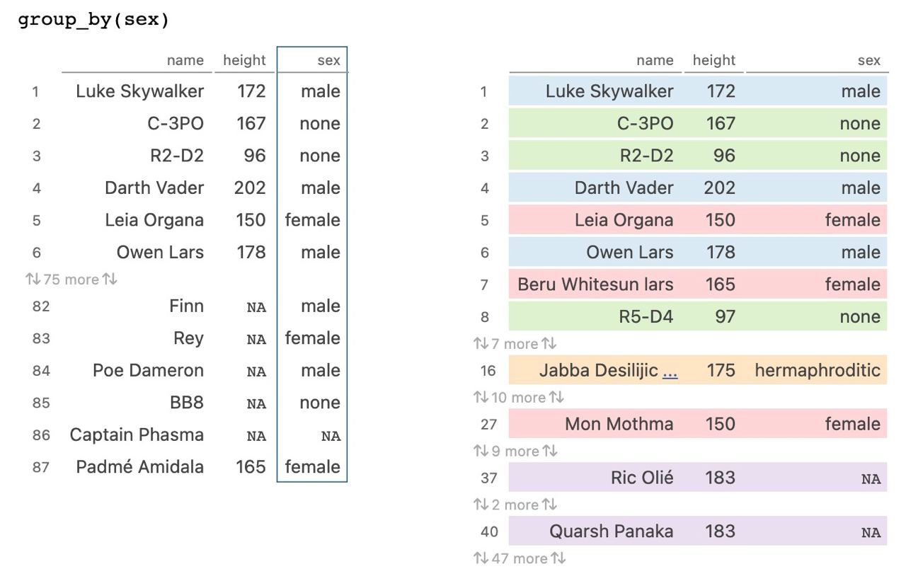
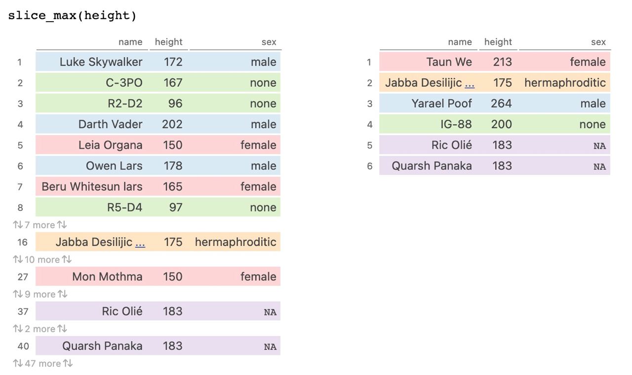
The web https://tidydatatutor.com/ allows to visualize the operations of {tidyverse} (doing with the old pipe %>%)
group_by()
Important
You should always remember to make ungroup to remove the created group variable.
The “new” version of {dplyr} now allows to include the group variable in the call to many functions with the argument by = ... or .by = ....
# A tibble: 5 × 6
name height mass hair_color skin_color eye_color
<chr> <int> <dbl> <chr> <chr> <chr>
1 Yarael Poof 264 NA none white yellow
2 IG-88 200 140 none metal red
3 Taun We 213 NA none grey black
4 Jabba Desilijic Tiure 175 1358 <NA> green-tan, brown orange
5 Gregar Typho 185 85 black dark brown Row-by-row: rowwise()
A very useful option used before an operation is also rowwise(): every operation that comes afterwards will be applied on each row separately. For example, let’s define a dummy set of grades.
If we apply the average directly the value will be identical since it has done the global average, but we would like to get an average per record. For that we will use rowwise().
Summary: summarise()
Finally we have summarise(), which will allow us to get statistical summaries. For example, let’s calculate the average of the heights.
# A tibble: 1 × 1
ave_height
<dbl>
1 175.Be careful
Notice that mutate() returns as many rows as original records, while with summarise() it calculates a new summary dataset, only including what is indicated.
Summary: summarise()
If we also combine this with the grouping of group_by() or .by = ..., in a few lines of code you can get disaggregated statistics.
Summary: reframe()
In the new {dplyr} they have included reframe() to avoid summarise() problems when we return more than one value per variable in more complex summaries.
Warning: Returning more (or less) than 1 row per `summarise()` group was deprecated in
dplyr 1.1.0.
ℹ Please use `reframe()` instead.
ℹ When switching from `summarise()` to `reframe()`, remember that `reframe()`
always returns an ungrouped data frame and adjust accordingly.# A tibble: 5 × 1
`quantile(mass)`
<dbl>
1 15
2 55.6
3 79
4 84.5
5 1358 across()
One trick is to make use of selectors across() and where(). The former allows us to act on several columns by name (with mutate() or summarise()).
# A tibble: 5 × 2
sex ave$height $mass
<chr> <dbl> <dbl>
1 male 179. 80.2
2 none 131. 69.8
3 female 172. 54.7
4 hermaphroditic 175 1358
5 <NA> 175 81 The second, where(), allows us to do the same but selecting by type.
# A tibble: 6 × 5
sex gender height mass birth_year
<chr> <chr> <dbl> <dbl> <dbl>
1 male masculine 179. 80.2 84.8
2 none masculine 140 69.8 53.3
3 female feminine 172. 54.7 47.2
4 hermaphroditic masculine 175 1358 600
5 <NA> <NA> 175 81 NaN
6 none feminine 96 NaN NaN 💻 It’s your turn
Try to perform the following exercises without looking at the solutions
📝 Calculate how many characters there are of each species, ordered from most to least frequent.
📝 After eliminating missing variables for weight and height, add a new variable to calculate the BMI of each character, and determine the average BMI of our characters disaggregated by gender.
📝 Obtain the youngest character for each gender.
📝 Get the age of the youngest and oldest character of each sex.
🐣 Case study I: billboard
We are going to do a summary of what we learned in {tidyverse} with the billboard table of the {tidyr} package. The dataset represents something similar to the top 40 (but American version and a top 100 instead of 40): for each artist and song we store the date when it entered the ranking, and the position it occupied in the ranking in each of the weeks (wk1, wk2, …).
# A tibble: 317 × 8
artist track date.entered wk1 wk2 wk3 wk4 wk5
<chr> <chr> <date> <dbl> <dbl> <dbl> <dbl> <dbl>
1 2 Pac Baby Don't Cry (Ke… 2000-02-26 87 82 72 77 87
2 2Ge+her The Hardest Part O… 2000-09-02 91 87 92 NA NA
3 3 Doors Down Kryptonite 2000-04-08 81 70 68 67 66
4 3 Doors Down Loser 2000-10-21 76 76 72 69 67
5 504 Boyz Wobble Wobble 2000-04-15 57 34 25 17 17
6 98^0 Give Me Just One N… 2000-08-19 51 39 34 26 26
7 A*Teens Dancing Queen 2000-07-08 97 97 96 95 100
8 Aaliyah I Don't Wanna 2000-01-29 84 62 51 41 38
9 Aaliyah Try Again 2000-03-18 59 53 38 28 21
10 Adams, Yolanda Open My Heart 2000-08-26 76 76 74 69 68
# ℹ 307 more rowsTry to answer the questions posed in the workbook.
🐣 Case study II: soccer
Let’s continue practicing what we learned in {tidyverse} with the file futbol.csv, where we have data of the players of the 5 main men’s soccer leagues, from 2005 to 2019, compiling different statistics. The data has been extracted directly using the {worldfootballR} package, which allows us to extract data from https://www.fbref.com.
# A tibble: 40,393 × 16
season team league player country position date_birth minutes_playing
<dbl> <chr> <chr> <chr> <chr> <chr> <dbl> <dbl>
1 2005 Ajaccio Ligue 1 Djamel Ab… ALG MF 1986 30
2 2005 Ajaccio Ligue 1 Gaspar Az… POR DF 1975 1224
3 2005 Ajaccio Ligue 1 Yacine Be… ALG MF 1981 140
4 2005 Ajaccio Ligue 1 Nicolas B… FRA MF 1976 892
5 2005 Ajaccio Ligue 1 Marcelinh… BRA MF 1971 704
6 2005 Ajaccio Ligue 1 Cyril Cha… FRA FW 1979 1308
7 2005 Ajaccio Ligue 1 Xavier Co… FRA DF 1974 2734
8 2005 Ajaccio Ligue 1 Renaud Co… FRA MF 1980 896
9 2005 Ajaccio Ligue 1 Yohan Dem… FRA DF,MF 1978 2658
10 2005 Ajaccio Ligue 1 Christoph… FRA DF 1973 74
# ℹ 40,383 more rows
# ℹ 8 more variables: minutes_per_match_playing <dbl>, goals <dbl>,
# assist <dbl>, goals_minus_pk <dbl>, pk <dbl>, pk_attemp <dbl>,
# yellow_card <dbl>, red_card <dbl>🐣 Case study II: soccer
The variables capture the following information:
season,team,league: season, team and league.player,country,position,date_birth: name, country, position and birth of year of each player.minutes_playing,matches: total minutes playing and 90’ matches playedgoals,assist: goals and assists.pk,pk_attemp,goals_minus_pk: penalties, penalties attempted and goals excluding penalties.yellow_card,red_card: yellow/red cards.
🐣 Case study II: soccer
# A tibble: 40,393 × 16
season team league player country position date_birth minutes_playing
<dbl> <chr> <chr> <chr> <chr> <chr> <dbl> <dbl>
1 2005 Ajaccio Ligue 1 Djamel Ab… ALG MF 1986 30
2 2005 Ajaccio Ligue 1 Gaspar Az… POR DF 1975 1224
3 2005 Ajaccio Ligue 1 Yacine Be… ALG MF 1981 140
4 2005 Ajaccio Ligue 1 Nicolas B… FRA MF 1976 892
5 2005 Ajaccio Ligue 1 Marcelinh… BRA MF 1971 704
6 2005 Ajaccio Ligue 1 Cyril Cha… FRA FW 1979 1308
7 2005 Ajaccio Ligue 1 Xavier Co… FRA DF 1974 2734
8 2005 Ajaccio Ligue 1 Renaud Co… FRA MF 1980 896
9 2005 Ajaccio Ligue 1 Yohan Dem… FRA DF,MF 1978 2658
10 2005 Ajaccio Ligue 1 Christoph… FRA DF 1973 74
# ℹ 40,383 more rows
# ℹ 8 more variables: minutes_per_match_playing <dbl>, goals <dbl>,
# assist <dbl>, goals_minus_pk <dbl>, pk <dbl>, pk_attemp <dbl>,
# yellow_card <dbl>, red_card <dbl>
Try to answer the questions posed in the workbook.
🐣 Case study III: speechs
Although we cannot do arithmetic operations with them, some operations we can do with the text strings will be important. For that we will use the {stringr} package (within the same {lubridate} “universe of packages”).
The dataset will be discursos (speeches, extracted from https://github.com/lirondos/discursos-de-navidad) where are stored the christmas speeches of the heads of state of Spain from 1946 to 2021 (in dictatorship and in democracy)
Try to answer the questions posed in the workbook.
L5: loops
Coming back to R base: loops
Loops
Although in most occasions they can be replaced by other more efficient and readable structures, it is important to know one of the most famous control expressions: the loops.
for { }: allows [repeating the same code]{. hl-yellow} in a prefixed and known number of times.while { }: allows repeating the same code but in an undetermined number of times (until a condition is no longer fulfilled).
For loop
A for loop is a structure that allows to repeat a set of commands a finite, prefixed and known number of times given a set of indices.
Let’s define a vector x <- c(0, -7, 1, 4) and another empty variable y. After that we will define a for loop with for () { }: inside the brackets we will indicate an index and some values to traverse, inside the braces the code to execute in each iteration (in this case, fill y as x + 1).
For loop
Note that because R works in a default vector manner, the loop is the same as doing x + 1 directly.
For loop
Another common option is to indicate the indexes “automatically”: from the first 1 to the last (corresponding to the length of x length(x)).
For loop
Thus the general structure of a for-loop will always be as follows
In the case of for loops ALWAYS we know how many iterations we have (as many as there are elements in the set to be indexed).
Avoiding loop
As we have already learned with the {microbenchmark} package, we can check how loops are usually very inefficient (hence we should avoid them in most occasions)
For loop
We can see another example of a combining numbers and text loop: we define a vector of ages and names, and print the i-th name and age.
For loop
Although they are usually indexed with numeric vectors, loops can be indexed on any vector structure, regardless of the type of the set.
For + if-else
Let’s combine conditional structures and loops: using the swiss set of the {datasets} package, let’s assign NA if the fertility values are greater than 80.
While loop
Another way to create a loop is with the while { } structure, which will loop an unknown number of times, until a condition stops being met (in fact it may never end). For example, we will inialize a variable times <- 1, which we will increment at each step, and we will not exit the loop until times > 3.
While loop
A while loop will always look like this
While loop
What happens when the condition is never FALSE? Try it yourself
Warning
A while { } loop can be quite “dangerous” if we do not control well how to stop it.
While loop
We have two reserved commands to abort a loop or force it forward:
break: allows abort a loop even if its end has not been reached
While loop
We have two reserved commands to abort a loop or force it forward:
next: forces a loop to advance to the next iteration
💻 It’s your turn
Try to perform the following exercises without looking at the solutions
📝 Modify the code below to print a message on the screen if and only if all the data in airquality is for a month other than January.
📝 Modify the code below to store in a variable called temp_high a TRUE if any of the records has a temperature above 90 degrees Fahrenheit and FALSE in any other case.
📝 Modify the code below to design a for loop of 5 iterations that only loops through the first 5 odd (and at each step of the loop prints them)
🐣 Case study I: simulations
Try to answer the questions posed in the workbook. On it you will have to design some simulation studies using conditional loops and structures.
🐣 Case study II: Monty Hall problem
Imagine you are in a TV contest where you are given a choice of 3 doors: in one there is a millionaire prize and in the other 2 there is an oreo cookie.
Try to answer the questions posed in the workbook. On it you will have to design some simulation studies using conditional loops and structures.
L6: functions and joins
Coming back to R base: functions. Joins
Own functions
Not only can we use default functions that come already loaded in packages, we can also create our own functions to automate tasks. How to create our own function? Let’s look at its basic scheme:
Name: for example
name_fun(no spaces or strange characters). To the name we assign the reserved wordfunction().Define input arguments (inside
function()).Body of the function inside
{ }.We end the function with the output arguments with
return().
Own functions
arg1, arg2, ...: will be the input arguments, the arguments that the function takes to execute the code inside.code: lines of code that we want to execute the function.return(var_output): the output arguments will be entered.
Important
All variables that we define inside the function are LOCAL variables: they will only exist inside the function unless we specify otherwise.
Own functions
Let’s look at a very simple example of a function for calculating the area of a rectangle.
Since the area of a rectangle is calculated as the product of its sides, we will need just that, its sides: those will be the input arguments and the value to return will be just its area (\(side_1 * side_2\)).
Own functions
We can also make a direct definition of variables without storing along the way.
Own functions
Consejo
Although it is not necessary, it is recommendable to make explicit the calling of the arguments, specifying in the code what value is for each argument so that it does not depend on its order, making the code more readable.
Default arguments
Imagine now that we realize that 90% of the time we use such a function to default calculate the area of a square (i.e., we only need one side). To do this, we can define default arguments in the function: they will take that value unless we assign another one.
Why not assign side_2 = side_1 default, to save lines of code and time?
Default arguments
Now default the second side will be equal to the first (if added it will use both).
Multiple outputs
Let’s complicate the function a bit and add in the output the values of each side, labeled side_1 and side_2, packing the output in a vector.
Multiple outputs
We can complicate the output a little more by adding a fourth variable that tells us, depending on the arguments, whether rectangle or square, having to add a character (or logic) variable in the output.
compute_area <- function(side_1, side_2 = side_1) {
# Code
area <- side_1 * side_2
# Output
return(c("area" = area, "side_1" = side_1, "side_2" = side_2,
"type" = if_else(side_1 == side_2, "square", "rectangle")))
}
compute_area(5, 3) area side_1 side_2 type
"15" "5" "3" "rectangle" Problem: when trying to put numbers and text together, it converts everything to numbers. We could store it all in a tibble() as we have learned or in an object known in R as lists (we will see it later).
Order of arguments
Before we did not care about the order of the arguments, but now the order of the input arguments matters, since we include side_1 and side_2 in the output.
Generating knowledge
It seems silly what we have done but we have crossed an important frontier: we have gone from consuming knowledge (code from other packages, elaborated by others), to generating knowledge, creating our own functions.
Functions are going to be key in your day-to-day work because they will allow you to automate code that you are going to repeat over and over again: by packaging that code under an alias (function name) you will be able to use it over and over again without programming it (so doing twice as much work will not imply working twice as much)
Local vs global variables
An important aspect to think about with functions: what happens if we name a variable inside a function to which we have forgotten to assign a value inside the function.
Local vs global variables
If a variable is already defined outside the function (global environment), and is also used inside changing its value, the value only changes inside but not in the global environment.
Local vs global variables
If we want it to change locally as well as globally we must use the double assignment (<<-).
💻 It’s your turn
Try to perform the following exercises without looking at the solutions
📝 Modify the code below to define a function called sum_function, so that given two elements, it returns their sum.
📝 Modify the code below to define a function called product_function, so that given two elements, it returns their product, but by default it calculates the square
📝 Define a function called equal_names that, given two names, tells us if they are equal or not. Do this by considering case-sensitive, and case-insensitive. Use the {stringr} package.
Código
# Case-sensitive
equal_names <- function(person_1, person_2) {
return(person_1 == person_2)
}
equal_names("Javi", "javi")
equal_names("Javi", "Lucía")
# Case-insensitive
library(stringr)
equal_names <- function(person_1, person_2) {
return(str_equal(person_1, person_2, ignore_case = TRUE))
# other option
# return(str_to_lower(person_1) == str_to_lower(person_2))
# other option
# return(str_to_upper(person_1) == str_to_upper(person_2))
}
equal_names("Javi", "javi")
equal_names("Javi", "Lucía")📝 Create a function called compute_BMI that, given two arguments (weight and height in meters) and a name, returns a list with the BMI (\(weight/(height^2)\)) and the name.
📝 Repeat the previous exercise but with another optional argument called units (by default, units = “meters”). Develop the function so that it does the right thing if units = “meters” and if units = “centimeters”.
📝 Create a fictitious tibble of 7 persons, with three variables (invent name, and simulate weight, height in centimeters), and apply the defined function so that we obtain a fourth column with their BMI.
📝 Create a function called shortcut that has two numeric arguments x and y. If both are equal, you should return equal and have the function terminate automatically (think about when a function exits). WARNING: x and y could be vectors. If they are different (of equal length) calculate the proportion of different elements. If they are different (being of different length), it returns the elements that are not common.
🐣 Case study I: converter
To practice with functions we are going to create a complete temperature converter that, given a temperature in Fahrenheit, Celsius or Kelvin, converts it to any of the others.
Try to answer the questions posed in the workbook
Joins
When working with data we will not always have the information in a single table, and sometimes, we will be interested in cross-referencing information from different sources.
Joins
inner_join(): only records with id in both tables survive.full_join(): keeps all records in both tables.left_join(): keeps all the records of the first table, and looks for which ones have id also in the second one (in case of not having it, it fills with NA the fields of the 2nd table).right_join(): keeps all records in the second table, and searches which ones have id also in the first one.
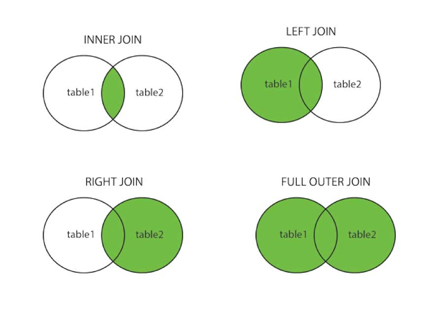
Joins
Let’s test the various joins with a simple example
left_join()
Imagine that we want to incorporate to tb_1 the information from table_2, identifying the records by the key column (by = "key", the column it has to cross): we want to keep all the records of the first table and look for which ones have the same value in key also in the second one.
left_join()
# A tibble: 3 × 3
key val_x val_y
<dbl> <chr> <chr>
1 1 x1 y1
2 2 x2 y2
3 3 x3 <NA> Notice that the records in the first one whose key was not found in the second one has given them the value of absent.
right_join()
The right_join() will perform the opposite operation: we will now incorporate to tb_2 the information from table_2, identifying the records by the key column: we want to keep all the records of the second one and look for which ones have id (same value in key) also in the first table.
right_join()
# A tibble: 3 × 3
key val_x val_y
<dbl> <chr> <chr>
1 1 x1 y1
2 2 x2 y2
3 4 <NA> y3 Notice that now the records of the second one whose key was not found in the first one are the ones given the value of absent.
keys and suffixes
The key columns we will use for the crossover will not always be named the same.
by = c("key_2" = "key_2"): we will indicate in which column of each table are the keys that we are going to cross.
keys and suffixes
We can also cross over several columns at the same time (it will interpret as equal record the one that has the same set of keys), with by = c("var1_t1" = "var1_t2", "var2_t1" = "var2_t2", ...). Let’s modify the previous example
keys and suffixes
It could also happen that when crossing two tables, there are columns of values named the same
keys and suffixes
This suffix can be specified in the optional argument suffix = ..., which allows us to distinguish the variables of one table from another.
full_join()
The two previous cases form what is known as outer joins: crosses where observations are kept that appear in at least one table. The third outer join is known as full_join() which will keep observations from both tables, adding rows that do not match the other table.
inner_join()
Opposite the outer join is what is known as inner join, with inner_join(): a join in which only the observations that appear in both tables are kept, only those records that are patched are kept.
inner_join()
Note that in terms of records, inner_join if it is commutative, we don’t care about the order of the tables: the only thing that changes is the order of the columns it adds.
semi/anti_join()
Finally we have two interesting tools to filter (not cross) records: semi_join() and anti_join(). The semi join leaves us in the first table the records whose key is also in the second table (like an inner join but without adding the info from the second table). And the second one, the anti join, does just the opposite (those that are not).
💻 It’s your turn
For the exercises we will use the tables available in the package {nycflights13}.
- airlines: name of airlines (with their abbreviation).
- airports: airport data (names, longitude, latitude, altitude, etc).
- flights, planes: flight and aircraft data.
- weather: hourly weather data.
💻 It’s your turn
📝 From package {nycflights13} incorporates into the flights table the airline data in airlines. We want to maintain all flight records, adding the airline information to the airlines table.
📝 To the table obtained from the crossing of the previous section, include the data of the aircraft in planes, but including only those flights for which we have information on their aircraft (and vice versa).
📝 Repeat the previous exercise but keeping both year variables (in one is the year of flight, in the other is the year of construction of the aircraft), and distinguishing them from each other
📝 To the table obtained from the previous exercise includes the longitude and latitude of the airports in airports, distinguishing between the latitude/longitude of the airport at destination and at origin.
📝 Filter from airports only those airports from which flights depart. Repeat the process filtering only those airports where flights arrive.
🐣 Case study II: Beatles
We will use to practice simple joins the band_members and band_instruments datasets already included in the {dplyr} package.
# A tibble: 3 × 2
name band
<chr> <chr>
1 Mick Stones
2 John Beatles
3 Paul Beatles# A tibble: 3 × 2
name plays
<chr> <chr>
1 John guitar
2 Paul bass
3 Keith guitar
Try to answer the questions posed in the workbook
🐣 Case study III: income by municipalities
In the file municipios.csv we have stored the information of the municipalities of Spain as of 2019.
The variable
LAU_coderepresents the code as local administrative unit in the EU (see more at https://ec.europa.eu/eurostat/web/nuts/local-administrative-units).The variable
codigo_ineis formed by joining the province code and the community code (each province has a code from 1 to 52, it does not depend on the ccaa).
# A tibble: 8,212 × 8
codauto ine.ccaa.name cpro ine.prov.name cmun name LAU_CODE codigo_ine
<chr> <chr> <chr> <chr> <chr> <chr> <chr> <chr>
1 01 Andalucía 04 Almería 001 Abla 04001 04001
2 01 Andalucía 04 Almería 002 Abrucena 04002 04002
3 01 Andalucía 04 Almería 003 Adra 04003 04003
4 01 Andalucía 04 Almería 004 Albanchez 04004 04004
5 01 Andalucía 04 Almería 005 Alboloduy 04005 04005
6 01 Andalucía 04 Almería 006 Albox 04006 04006
7 01 Andalucía 04 Almería 007 Alcolea 04007 04007
8 01 Andalucía 04 Almería 008 Alcóntar 04008 04008
9 01 Andalucía 04 Almería 009 Alcudia … 04009 04009
10 01 Andalucía 04 Almería 010 Alhabia 04010 04010
# ℹ 8,202 more rows🐣 Case study III: income by municipalities
On the other hand, in the file renta_mun we have the average per capita income of each administrative unit (municipalities, districts, provinces, autonomous communities,…) for different years.
# A tibble: 55,273 × 7
Unidad `2019` `2018` `2017` `2016` `2015` codigo_ine
<chr> <dbl> <dbl> <dbl> <dbl> <dbl> <chr>
1 44001 Ababuj NA NA NA NA NA 44001
2 4400101 Ababuj distrito 01 NA NA NA NA NA 4400101
3 4400101001 Ababuj sección 01001 NA NA NA NA NA 4400101001
4 40001 Abades 11429 10731 10314 9816 9904 40001
5 4000101 Abades distrito 01 11429 10731 10314 9816 9904 4000101
6 4000101001 Abades sección 01001 11429 10731 10314 9816 9904 4000101001
7 10001 Abadía 8954 8589 8207 7671 8416 10001
8 1000101 Abadía distrito 01 8954 8589 8207 7671 8416 1000101
9 1000101001 Abadía sección 01001 8954 8589 8207 7671 8416 1000101001
10 27001 Abadín 10791 10258 9762 9478 9116 27001
# ℹ 55,263 more rows🐣 Case study III: income by municipalities
Before we start let’s normalize variable names using clean_names() from the {janitor} package.
Try to answer the questions posed in the workbook
L7: import/exports
Import and export data
Import/export
So far we have only used data already loaded in packages but many times we will need to import data externally. One of the main strengths of R is that we can import data very easily in different formats:
R native formats:
.rda,.RDataand.rdsformats.Rectangular (tabular) data:
.csvand.tsvformatsUntabulated data:
.txtformat.Data in excel:
.xlsand.xlsxformatsData from SAS/Stata/SPSS:
.sas7bdat,.savand.datformatsData from Google Drive
Data from API’s: aemet, catastro, twitter, spotify, etc.
R native formats
The simplest files to import into R (and which usually take up less disk space) are its own native extensions: files in .RData, .rda and .rds formats. To load the former we simply need to use the native function load() by providing it the file path.
RDatafile: we are going to import the fileworld_bank_pop.RData, which includes the datasetworld_bank_pop
# A tibble: 1,064 × 20
country indicator `2000` `2001` `2002` `2003` `2004` `2005` `2006`
<chr> <chr> <dbl> <dbl> <dbl> <dbl> <dbl> <dbl> <dbl>
1 ABW SP.URB.TOTL 4.16e4 4.20e+4 4.22e+4 4.23e+4 4.23e+4 4.24e+4 4.26e+4
2 ABW SP.URB.GROW 1.66e0 9.56e-1 4.01e-1 1.97e-1 9.46e-2 1.94e-1 3.67e-1
3 ABW SP.POP.TOTL 8.91e4 9.07e+4 9.18e+4 9.27e+4 9.35e+4 9.45e+4 9.56e+4
4 ABW SP.POP.GROW 2.54e0 1.77e+0 1.19e+0 9.97e-1 9.01e-1 1.00e+0 1.18e+0
5 AFE SP.URB.TOTL 1.16e8 1.20e+8 1.24e+8 1.29e+8 1.34e+8 1.39e+8 1.44e+8
6 AFE SP.URB.GROW 3.60e0 3.66e+0 3.72e+0 3.71e+0 3.74e+0 3.81e+0 3.81e+0
7 AFE SP.POP.TOTL 4.02e8 4.12e+8 4.23e+8 4.34e+8 4.45e+8 4.57e+8 4.70e+8
8 AFE SP.POP.GROW 2.58e0 2.59e+0 2.61e+0 2.62e+0 2.64e+0 2.67e+0 2.70e+0
9 AFG SP.URB.TOTL 4.31e6 4.36e+6 4.67e+6 5.06e+6 5.30e+6 5.54e+6 5.83e+6
10 AFG SP.URB.GROW 1.86e0 1.15e+0 6.86e+0 7.95e+0 4.59e+0 4.47e+0 5.03e+0
# ℹ 1,054 more rows
# ℹ 11 more variables: `2007` <dbl>, `2008` <dbl>, `2009` <dbl>, `2010` <dbl>,
# `2011` <dbl>, `2012` <dbl>, `2013` <dbl>, `2014` <dbl>, `2015` <dbl>,
# `2016` <dbl>, `2017` <dbl>R native formats
.rdafile: we will import the airquality dataset fromairquality.rda
# A tibble: 153 × 6
Ozone Solar.R Wind Temp Month Day
<int> <int> <dbl> <int> <int> <int>
1 41 190 7.4 67 5 1
2 36 118 8 72 5 2
3 12 149 12.6 74 5 3
4 18 313 11.5 62 5 4
5 NA NA 14.3 56 5 5
6 28 NA 14.9 66 5 6
7 23 299 8.6 65 5 7
8 19 99 13.8 59 5 8
9 8 19 20.1 61 5 9
10 NA 194 8.6 69 5 10
# ℹ 143 more rowsR native formats
Note that files loaded with load() are automatically loaded into the environment (with the originally saved name), and not only datasets can be loaded: load() allows us to load multiple objetcs (not only a tabular data)
Native .rda and .RData files are a properly way to save your environment.
R native formats
.rdsfiles: for this type we must usereadRDS(), and we need to incorporate a argumentfilewith the path. In this case we are going to import lung cancer data from the North Central Cancer Treatment Group. Note that now .rds import files are a unique database
# A tibble: 228 × 10
inst time status age sex ph.ecog ph.karno pat.karno meal.cal wt.loss
<dbl> <dbl> <dbl> <dbl> <dbl> <dbl> <dbl> <dbl> <dbl> <dbl>
1 3 306 2 74 1 1 90 100 1175 NA
2 3 455 2 68 1 0 90 90 1225 15
3 3 1010 1 56 1 0 90 90 NA 15
4 5 210 2 57 1 1 90 60 1150 11
5 1 883 2 60 1 0 100 90 NA 0
6 12 1022 1 74 1 1 50 80 513 0
7 7 310 2 68 2 2 70 60 384 10
8 11 361 2 71 2 2 60 80 538 1
9 1 218 2 53 1 1 70 80 825 16
10 7 166 2 61 1 2 70 70 271 34
# ℹ 218 more rowsImportant
The paths must always be without spaces, ñ, or accents.
Tabular data: readr
The {readr} package within the {tidyverse} environment contains several useful functions for loading rectangular data (without formatting).
read_csv():.csvfiles whose separator is commaread_csv2(): semicolonread_tsv(): tabulator.read_table(): space.read_delim(): generic function for character delimited files.
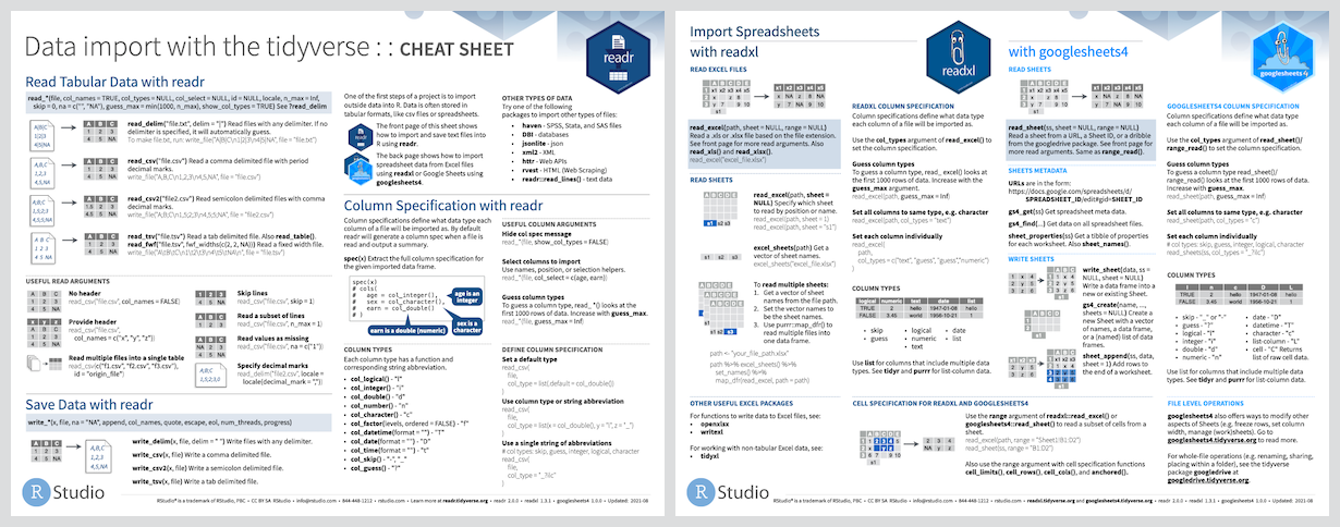
All of them need as argument the file path plus other optional (skip header or not, decimals, etc). See more at https://readr.tidyverse.org/
Tabular data (.csv, .tsv)
The main advantage of {readr} is that it automates formatting to go from a flat (unformatted) file to a tibble (in rows and columns, with formatting).
- File
.csv: withread_csv()we will load comma separated files, passing as argument the path infile = .... Let’s import thechickens.csvdataset (about cartoon chickens, why not). If you look at the output it gives us the type of variables.
# A tibble: 5 × 4
chicken sex eggs_laid motto
<chr> <chr> <dbl> <chr>
1 Foghorn Leghorn rooster 0 That's a joke, ah say, that's a jok…
2 Chicken Little hen 3 The sky is falling!
3 Ginger hen 12 Listen. We'll either die free chick…
4 Camilla the Chicken hen 7 Bawk, buck, ba-gawk.
5 Ernie The Giant Chicken rooster 0 Put Captain Solo in the cargo hold. Tabular data (.csv, .tsv)
The variable format will normally be done automatically by read_csv(), and we can query it with spec().
Tabular data (.csv, .tsv)
Although it usually does it well automatically we can specify the format explicitly in col_types = list() (in list format, with col_xxx() for each type of variable, for example eggs_laid will be imported as character).
chickens <-
read_csv(file = "./data/chickens.csv",
col_types = list(col_character(), col_character(),
col_character(), col_character()))
chickens# A tibble: 5 × 4
chicken sex eggs_laid motto
<chr> <chr> <chr> <chr>
1 Foghorn Leghorn rooster 0 That's a joke, ah say, that's a jok…
2 Chicken Little hen 3 The sky is falling!
3 Ginger hen 12 Listen. We'll either die free chick…
4 Camilla the Chicken hen 7 Bawk, buck, ba-gawk.
5 Ernie The Giant Chicken rooster 0 Put Captain Solo in the cargo hold. Tabular data (.csv, .tsv)
We can even indicate that variables we want to select (without occupying memory), by indicating it in col_select = ... (in list format, with col_select = ...).
Untabulated data (.txt)
What happens when the separator is not correct?
If we use read_csv() it expects the separator between columns to be a comma but, as you can see with the following .txt, it interprets everything as a single column: has no comma and does not know where to separate
[1] 10 1# A tibble: 10 × 1
`UCC PAY LAZ KPK RT COF BIH DII ENG ACU Rank Team Conf`
<chr>
1 1 1 1 1 1 1 1 1 1 1 1 Ohio St B10
2 2 2 2 2 2 2 2 2 4 2 2 Oregon P12
3 3 4 3 4 3 4 3 4 2 3 3 Alabama SEC
4 4 3 4 3 4 3 5 3 3 4 4 TCU B12
5 6 6 6 5 5 7 6 5 6 11 5 Michigan St B10
6 7 7 7 6 7 6 11 8 7 8 6 Georgia SEC
7 5 5 5 7 6 8 4 6 5 5 7 Florida St ACC
8 8 8 9 9 10 5 7 7 10 7 8 Baylor B12
9 9 11 8 13 11 11 12 9 14 9 9 Georgia Tech ACC
10 13 10 13 11 8 9 10 11 9 10 10 Mississippi SEC Untabulated data (.txt)
To do this we have.
read_csv2()when the separator is semicolon,read_tsv()when the is a tab andread_table()when the is a space.read_delim()in general.
# A tibble: 10 × 13
UCC PAY LAZ KPK RT COF BIH DII ENG ACU Rank Team Conf
<dbl> <dbl> <dbl> <dbl> <dbl> <dbl> <dbl> <dbl> <dbl> <dbl> <dbl> <chr> <chr>
1 1 1 1 1 1 1 1 1 1 1 1 Ohio St
2 2 2 2 2 2 2 2 2 4 2 2 Oreg… P12
3 3 4 3 4 3 4 3 4 2 3 3 Alab… SEC
4 4 3 4 3 4 3 5 3 3 4 4 TCU B12
5 6 6 6 5 5 7 6 5 6 11 5 Mich… St
6 7 7 7 6 7 6 11 8 7 8 6 Geor… SEC
7 5 5 5 7 6 8 4 6 5 5 7 Flor… St
8 8 8 9 9 10 5 7 7 10 7 8 Bayl… B12
9 9 11 8 13 11 11 12 9 14 9 9 Geor… Tech
10 13 10 13 11 8 9 10 11 9 10 10 Miss… SEC Excel data (.xls, .xlsx)
Another key import package will be the {readxl} package for importing data from Excel. Three functions will be key:
read_xls()specific to.xls,read_xlsx()specific to.xlsx.read_excel(): for both.xlsand.xlsx.
We are going to import deaths.xlsx with celebrity death records.
# A tibble: 18 × 6
`Lots of people` ...2 ...3 ...4 ...5 ...6
<chr> <chr> <chr> <chr> <chr> <chr>
1 simply cannot resist writing <NA> <NA> <NA> <NA> some…
2 at the top <NA> of thei…
3 or merging <NA> <NA> <NA> cells
4 Name Profession Age Has … Date… Date…
5 David Bowie musician 69 TRUE 17175 42379
6 Carrie Fisher actor 60 TRUE 20749 42731
7 Chuck Berry musician 90 TRUE 9788 42812
8 Bill Paxton actor 61 TRUE 20226 42791
9 Prince musician 57 TRUE 21343 42481
10 Alan Rickman actor 69 FALSE 16854 42383
11 Florence Henderson actor 82 TRUE 12464 42698
12 Harper Lee author 89 FALSE 9615 42419
13 Zsa Zsa Gábor actor 99 TRUE 6247 42722
14 George Michael musician 53 FALSE 23187 42729
15 Some <NA> <NA> <NA> <NA> <NA>
16 <NA> also like to write stuff <NA> <NA> <NA> <NA>
17 <NA> <NA> at t… bott… <NA> <NA>
18 <NA> <NA> <NA> <NA> <NA> too! Excel data (.xls, .xlsx)
# A tibble: 6 × 6
`Lots of people` ...2 ...3 ...4 ...5 ...6
<chr> <chr> <chr> <chr> <chr> <chr>
1 simply cannot resist writing <NA> <NA> <NA> <NA> some not…
2 at the top <NA> of their sp…
3 or merging <NA> <NA> <NA> cells
4 Name Profession Age Has kids Date of birth Date of …
5 David Bowie musician 69 TRUE 17175 42379
6 Carrie Fisher actor 60 TRUE 20749 42731 One thing that is very common misfortune is that there is some kind of comment or text at the beginning of the file, having to skip those rows.
Excel data (.xls, .xlsx)
We can skip these rows directly in the load with skip = ... (indicating the number of rows to skip).
# A tibble: 14 × 6
Name Profession Age `Has kids` `Date of birth` `Date of death`
<chr> <chr> <chr> <chr> <dttm> <chr>
1 David Bowie musician 69 TRUE 1947-01-08 00:00:00 42379
2 Carrie Fisher actor 60 TRUE 1956-10-21 00:00:00 42731
3 Chuck Berry musician 90 TRUE 1926-10-18 00:00:00 42812
4 Bill Paxton actor 61 TRUE 1955-05-17 00:00:00 42791
5 Prince musician 57 TRUE 1958-06-07 00:00:00 42481
6 Alan Rickman actor 69 FALSE 1946-02-21 00:00:00 42383
7 Florence Hen… actor 82 TRUE 1934-02-14 00:00:00 42698
8 Harper Lee author 89 FALSE 1926-04-28 00:00:00 42419
9 Zsa Zsa Gábor actor 99 TRUE 1917-02-06 00:00:00 42722
10 George Micha… musician 53 FALSE 1963-06-25 00:00:00 42729
11 Some <NA> <NA> <NA> NA <NA>
12 <NA> also like… <NA> <NA> NA <NA>
13 <NA> <NA> at t… bottom, NA <NA>
14 <NA> <NA> <NA> <NA> NA too! Excel data (.xls, .xlsx)
In addition with col_names = ... we can already rename the columns in the import (if provide names assumes 1st line already as a data)
deaths <-
read_xlsx(path = "./data/deaths.xlsx", skip = 5,
col_names = c("name", "profession", "age", "kids", "birth", "death"))
deaths# A tibble: 14 × 6
name profession age kids birth death
<chr> <chr> <chr> <chr> <dttm> <chr>
1 David Bowie musician 69 TRUE 1947-01-08 00:00:00 42379
2 Carrie Fisher actor 60 TRUE 1956-10-21 00:00:00 42731
3 Chuck Berry musician 90 TRUE 1926-10-18 00:00:00 42812
4 Bill Paxton actor 61 TRUE 1955-05-17 00:00:00 42791
5 Prince musician 57 TRUE 1958-06-07 00:00:00 42481
6 Alan Rickman actor 69 FALSE 1946-02-21 00:00:00 42383
7 Florence Henderson actor 82 TRUE 1934-02-14 00:00:00 42698
8 Harper Lee author 89 FALSE 1926-04-28 00:00:00 42419
9 Zsa Zsa Gábor actor 99 TRUE 1917-02-06 00:00:00 42722
10 George Michael musician 53 FALSE 1963-06-25 00:00:00 42729
11 Some <NA> <NA> <NA> NA <NA>
12 <NA> also like to write … <NA> <NA> NA <NA>
13 <NA> <NA> at t… bott… NA <NA>
14 <NA> <NA> <NA> <NA> NA too! Excel data (.xls, .xlsx)
Sometimes Excel dates are incorrectly formatted (surprise): we can use convertToDate() from the {openxlsx} package to convert it.
# A tibble: 14 × 6
name profession age kids birth death
<chr> <chr> <chr> <chr> <dttm> <date>
1 David Bowie musician 69 TRUE 1947-01-08 00:00:00 2016-01-10
2 Carrie Fisher actor 60 TRUE 1956-10-21 00:00:00 2016-12-27
3 Chuck Berry musician 90 TRUE 1926-10-18 00:00:00 2017-03-18
4 Bill Paxton actor 61 TRUE 1955-05-17 00:00:00 2017-02-25
5 Prince musician 57 TRUE 1958-06-07 00:00:00 2016-04-21
6 Alan Rickman actor 69 FALSE 1946-02-21 00:00:00 2016-01-14
7 Florence Henderson actor 82 TRUE 1934-02-14 00:00:00 2016-11-24
8 Harper Lee author 89 FALSE 1926-04-28 00:00:00 2016-02-19
9 Zsa Zsa Gábor actor 99 TRUE 1917-02-06 00:00:00 2016-12-18
10 George Michael musician 53 FALSE 1963-06-25 00:00:00 2016-12-25
11 Some <NA> <NA> <NA> NA NA
12 <NA> also like to w… <NA> <NA> NA NA
13 <NA> <NA> at t… bott… NA NA
14 <NA> <NA> <NA> <NA> NA NA Excel data (.xls, .xlsx)
We can also load an Excel with several sheets: to indicate the sheet (either by its name or by its number) we will use the argument sheet = ....
# A tibble: 32 × 11
mpg cyl disp hp drat wt qsec vs am gear carb
<dbl> <dbl> <dbl> <dbl> <dbl> <dbl> <dbl> <dbl> <dbl> <dbl> <dbl>
1 21 6 160 110 3.9 2.62 16.5 0 1 4 4
2 21 6 160 110 3.9 2.88 17.0 0 1 4 4
3 22.8 4 108 93 3.85 2.32 18.6 1 1 4 1
4 21.4 6 258 110 3.08 3.22 19.4 1 0 3 1
5 18.7 8 360 175 3.15 3.44 17.0 0 0 3 2
6 18.1 6 225 105 2.76 3.46 20.2 1 0 3 1
7 14.3 8 360 245 3.21 3.57 15.8 0 0 3 4
8 24.4 4 147. 62 3.69 3.19 20 1 0 4 2
9 22.8 4 141. 95 3.92 3.15 22.9 1 0 4 2
10 19.2 6 168. 123 3.92 3.44 18.3 1 0 4 4
# ℹ 22 more rowsExcel data (.xls, .xlsx)
We can even indicate the range of cells to load with range = ....
Import from SAS/STATA/SPSS
The {haven} package within the tidyverse orbit will allow us to import files from the 3 most important payment software: SAS, SPSS and Stata.
Export
In the same way that we can import we can also export
- exported in
.RData(recommended option for variables stored inR). Remember that this extension can only be used inR. To do so, just usesave(object, file = path).
Export
In the same way that we can import we can also export
- exported in
.RDatamultiple objects
Export
In the same way that we can import we can also export
- exported in
.csv. To do this we simply usewrite_csv(object, file = path).
Import from website
One of the main advantages of R is that we can make use of all the previous functions of import but directly from a web, without the need to perform the manual download: instead of passing it the local path we will indicate the link. For example, we are going to download the covid data from ISCIII (https://cnecovid.isciii.es/covid19/#documentaci%C3%B3n-y-datos)
# A tibble: 500 × 8
provincia_iso sexo grupo_edad fecha num_casos num_hosp num_uci num_def
<chr> <chr> <chr> <date> <dbl> <dbl> <dbl> <dbl>
1 A H 0-9 2020-01-01 0 0 0 0
2 A H 10-19 2020-01-01 0 0 0 0
3 A H 20-29 2020-01-01 0 0 0 0
4 A H 30-39 2020-01-01 0 0 0 0
5 A H 40-49 2020-01-01 0 0 0 0
6 A H 50-59 2020-01-01 0 0 0 0
7 A H 60-69 2020-01-01 0 0 0 0
8 A H 70-79 2020-01-01 0 0 0 0
9 A H 80+ 2020-01-01 0 0 0 0
10 A H NC 2020-01-01 0 0 0 0
# ℹ 490 more rowsImport from wikipedia
The {rvest} package, one of the most useful of {tidyverse} allows us to import directly from an html. For example, to export wikipedia tables just read_html() to import the html, html_element("table") to extract the table objects, and html_table() to convert the html table to tibble.
library(rvest)
wiki_jump <- 'https://en.wikipedia.org/wiki/Men%27s_long_jump_world_record_progression'
wiki_jump |> read_html() |>
html_element("table") |>
html_table()# A tibble: 19 × 5
Mark Wind Athlete Place Date
<chr> <chr> <chr> <chr> <chr>
1 7.61 m (24 ft 11+1⁄2 in) "" Peter O'Connor (IRE) Dublin, Ire… 5 Au…
2 7.69 m (25 ft 2+3⁄4 in) "" Edward Gourdin (USA) Cambridge, … 23 J…
3 7.76 m (25 ft 5+1⁄2 in) "" Robert LeGendre (USA) Paris, Fran… 7 Ju…
4 7.89 m (25 ft 10+1⁄2 in) "" DeHart Hubbard (USA) Chicago, Un… 13 J…
5 7.90 m (25 ft 11 in) "" Edward Hamm (USA) Cambridge, … 7 Ju…
6 7.93 m (26 ft 0 in) "0.0" Sylvio Cator (HAI) Paris, Fran… 9 Se…
7 7.98 m (26 ft 2 in) "0.5" Chuhei Nambu (JPN) Tokyo, Japan 27 O…
8 8.13 m (26 ft 8 in) "1.5" Jesse Owens (USA) Ann Arbor, … 25 M…
9 8.21 m (26 ft 11 in) "0.0" Ralph Boston (USA) Walnut, Uni… 12 A…
10 8.24 m (27 ft 1⁄4 in) "1.8" Ralph Boston (USA) Modesto, Un… 27 M…
11 8.28 m (27 ft 1+3⁄4 in) "1.2" Ralph Boston (USA) Moscow, Sov… 16 J…
12 8.31 m (27 ft 3 in) A "−0.1" Igor Ter-Ovanesyan (URS) Yerevan, So… 10 J…
13 8.33 m (27 ft 3+3⁄4 in)[2] "" Phil Shinnick (USA) Modesto, Un… 25 M…
14 8.31 m (27 ft 3 in) "0.0" Ralph Boston (USA) Kingston, J… 15 A…
15 8.34 m (27 ft 4+1⁄4 in) "1.0" Ralph Boston (USA) Los Angeles… 12 S…
16 8.35 m (27 ft 4+1⁄2 in)[5] "0.0" Ralph Boston (USA) Modesto, Un… 29 M…
17 8.35 m (27 ft 4+1⁄2 in) A "0.0" Igor Ter-Ovanesyan (URS) Mexico City… 19 O…
18 8.90 m (29 ft 2+1⁄4 in) A "2.0" Bob Beamon (USA) Mexico City… 18 O…
19 8.95 m (29 ft 4+1⁄4 in) "0.3" Mike Powell (USA) Tokyo, Japan 30 A…Import from google drive
Another option available (especially if we work with other people working) is to import from a Google Drive spreadsheet, making use of read_sheet() from the {googlesheets4} package.
The first time you will be asked for a tidyverse permission to interact with your drive
Import from API (owid)
Another interesting option is the data download from an API: an intermediary between an app or data provider and our R. For example, let’s load the {owidR} library, which allows us to download data from the web https://ourworldindata.org/. For example, the owid_covid() function loads without realizing it more than 400 000 records with more than 60 variables from 238 countries.
# A tibble: 7 × 67
iso_code continent location date total_cases new_cases
<chr> <chr> <chr> <IDate> <int> <int>
1 AFG Asia Afghanistan 2020-01-05 0 0
2 AFG Asia Afghanistan 2020-01-06 0 0
3 AFG Asia Afghanistan 2020-01-07 0 0
4 AFG Asia Afghanistan 2020-01-08 0 0
5 AFG Asia Afghanistan 2020-01-09 0 0
6 AFG Asia Afghanistan 2020-01-10 0 0
7 AFG Asia Afghanistan 2020-01-11 0 0
# ℹ 61 more variables: new_cases_smoothed <dbl>, total_deaths <int>,
# new_deaths <int>, new_deaths_smoothed <dbl>, total_cases_per_million <dbl>,
# new_cases_per_million <dbl>, new_cases_smoothed_per_million <dbl>,
# total_deaths_per_million <dbl>, new_deaths_per_million <dbl>,
# new_deaths_smoothed_per_million <dbl>, reproduction_rate <dbl>,
# icu_patients <int>, icu_patients_per_million <dbl>, hosp_patients <int>,
# hosp_patients_per_million <dbl>, weekly_icu_admissions <int>, …Import from API (aemet)
In many occasions to connect to the API we will first have to register and obtain a key, this is the case of the {climaemet} package to access Spanish meteorological data (https://opendata.aemet.es/centrodedescargas/inicio).
Once we have the API key we register it in our RStudio to be able to use it in the future.
library(climaemet)
# Api key
apikey <- "eyJhbGciOiJIUzI1NiJ9.eyJzdWIiOiJqYXZhbHYwOUB1Y20uZXMiLCJqdGkiOiI4YTU1ODUxMS01MTE3LTQ4MTYtYmM4OS1hYmVkNDhiODBkYzkiLCJpc3MiOiJBRU1FVCIsImlhdCI6MTY2NjQ2OTcxNSwidXNlcklkIjoiOGE1NTg1MTEtNTExNy00ODE2LWJjODktYWJlZDQ4YjgwZGM5Iiwicm9sZSI6IiJ9.HEMR77lZy2ASjmOxJa8ppx2J8Za1IViurMX3p1reVBU"
aemet_api_key(apikey, install = TRUE)Import from API (aemet)
With this package we can do a search for stations to know both its postal code and its identifier code within the AEMET network
# A tibble: 947 × 7
indicativo indsinop nombre provincia altitud longitud latitud
<chr> <chr> <chr> <chr> <dbl> <dbl> <dbl>
1 B013X "08304" ESCORCA, LLUC ILLES BA… 490 2.89 39.8
2 B051A "08316" SÓLLER, PUERTO ILLES BA… 5 2.69 39.8
3 B087X "" BANYALBUFAR ILLES BA… 60 2.51 39.7
4 B103B "99103" ANDRATX - SANT ELM ILLES BA… 52 2.37 39.6
5 B158X "" CALVIÀ, ES CAPDELLÀ ILLES BA… 50 2.47 39.6
6 B228 "08301" PALMA, PUERTO ILLES BA… 3 2.63 39.6
7 B236C "" PALMA, UNIVERSIDAD ILLES BA… 95 2.64 39.6
8 B248 "08303" SIERRA DE ALFABIA, BU… ILLES BA… 1030 2.71 39.7
9 B275E "08302" SON BONET, AEROPUERTO BALEARES 49 2.71 39.6
10 B278 "08306" PALMA DE MALLORCA, AE… ILLES BA… 8 2.74 39.6
# ℹ 937 more rowsImport from API (aemet)
For example, to get data from the station of the airport of El Prat, Barcelona, the code to provide is "0076", obtaining hourly data
# A tibble: 13 × 23
idema lon fint prec alt vmax vv dv lat dmax
<chr> <dbl> <dttm> <dbl> <dbl> <dbl> <dbl> <dbl> <dbl> <dbl>
1 0076 2.07 2024-11-02 23:00:00 0 4 5.7 3 360 41.3 350
2 0076 2.07 2024-11-03 00:00:00 0 4 5.7 3.9 360 41.3 360
3 0076 2.07 2024-11-03 01:00:00 0 4 6.2 3.6 10 41.3 20
4 0076 2.07 2024-11-03 02:00:00 0 4 5.1 3.8 360 41.3 10
5 0076 2.07 2024-11-03 03:00:00 0 4 5.7 4.3 360 41.3 350
6 0076 2.07 2024-11-03 04:00:00 0 4 6.7 4.6 360 41.3 20
7 0076 2.07 2024-11-03 05:00:00 0 4 7.2 5.7 360 41.3 10
8 0076 2.07 2024-11-03 06:00:00 0.2 4 7.2 5 360 41.3 20
9 0076 2.07 2024-11-03 07:00:00 0 4 6.2 4.6 10 41.3 10
10 0076 2.07 2024-11-03 08:00:00 0 4 11.3 5 30 41.3 10
11 0076 2.07 2024-11-03 09:00:00 0.1 4 10.3 4.5 40 41.3 30
12 0076 2.07 2024-11-03 10:00:00 9 4 6.2 3.4 290 41.3 320
13 0076 2.07 2024-11-03 11:00:00 0.1 4 10.3 3.5 360 41.3 20
# ℹ 13 more variables: ubi <chr>, pres <dbl>, hr <dbl>, stdvv <dbl>, ts <dbl>,
# pres_nmar <dbl>, tamin <dbl>, ta <dbl>, tamax <dbl>, tpr <dbl>, vis <dbl>,
# stddv <dbl>, inso <dbl>Importar from API (US census)
One of the most useful tools in recent years is known as {tidycensus}: a tool for facilitating the process of downloading census data for the United States from R.
get_decennial(): to access the census data (US Decennial Census), done every 10 years (years 2000, 2010 and 2020).get_acs(): to access the annual and quinquennial (5 years) ACS (American Community Survey) (census != survey)get_estimates(): to access the annual population, birth and death estimates (census != survey)get_pums(): to access the microdata (unaggregated data) of the ACS (anonymized at the individual level)get_flows(): to access the migration flow data.
Importar from API (US census)
For example, we will download the census data (get_decennial()) at the state level (geography = “state”) for the population (variable variables = “P001001”) for the year 2010 (see variables in tidycensus::load_variables()).
total_population_10 <-
get_decennial(geography = "state",
variables = "P001001",
year = 2010)
total_population_10# A tibble: 52 × 4
GEOID NAME variable value
<chr> <chr> <chr> <dbl>
1 01 Alabama P001001 4779736
2 02 Alaska P001001 710231
3 04 Arizona P001001 6392017
4 05 Arkansas P001001 2915918
5 06 California P001001 37253956
6 22 Louisiana P001001 4533372
7 21 Kentucky P001001 4339367
8 08 Colorado P001001 5029196
9 09 Connecticut P001001 3574097
10 10 Delaware P001001 897934
# ℹ 42 more rowsImport from API
Other options:
{chessR}: data from chess matches. See https://github.com/JaseZiv/chessR{spotifyr}: data from Spotify. See https://www.rcharlie.com/spotifyr/{gtrendsR}: data from Google Trends. See https://github.com/PMassicotte/gtrendsR{scholar}: data from https://github.com/jkeirstead/scholar
💻 Your turn
Try to solve the following exercises without looking at the solutions
📝 The who dataset we have used in previous exercises, export it to a native R format in the data folder of the project
📝 Loads the who dataset but from the data folder (import the file created in the previous exercise)
📝 Repeats the same (export and import) in 4 formats: .csv, .xlsx, .sav (spss) and .dta (stata)
Código
# csv
library(readr)
write_csv(who, file = "./data/who.csv")
who_data <- read_csv(file = "./data/who.csv")
# excel
library(openxlsx)
write.xlsx(who, file = "./data/who.xlsx")
who_data <- read_xlsx(path = "./data/who.xlsx")
# sas y stata
library(haven)
write_sav(who, path = "./data/who.sav")
who_data <- read_spss(path = "./data/who.sav")
write_dta(who, path = "./data/who.dta")
who_data <- read_dta(path = "./data/who.dta")🐣 Case study I: CIS feminism
We are going to put into practice the loading and preprocessing of a file generated by one of the most used software (SPSS). The file contains data from the CIS (Centro de Investigaciones Sociológicas) barometer «Perceptions on equality between men and women and gender stereotypes» (file extension .sav that you have in the subfolder CIS-feminism inside the data folder) whose sample work was carried out from November 6 to 14 (4000 interviews of both sexes over 16 years old in 1174 municipalities and 50 provinces).
Try to answer the questions posed in the workbook
L8: factors and lists
Handling with factors and lists
Lists
We have already seen that lists are an object in R that allows us to store collections of variables of different type (as with data.frame and tibble) but also different lengths, with totally heterogeneous structures (even a list can have inside it another list).
Lists
We can also make lists with other lists inside, so that to access each level we must use the [[]] operator.
[1] "list_1" "list_2"We are allowed to store n-dimensional data!
Lists
One of the disadvantages is that a list cannot be vectorized immediately, so any arithmetic operation applied to a list will give error.
Error in data/2: non-numeric argument to binary operatorLists
A more flexible and versatile option is to make use of the {purrr} package of the {tidyverse} environment.
This package is intended to mimic the functional programming of other languages such as Scala or Hadoop’s map-reduce strategy (from Google).
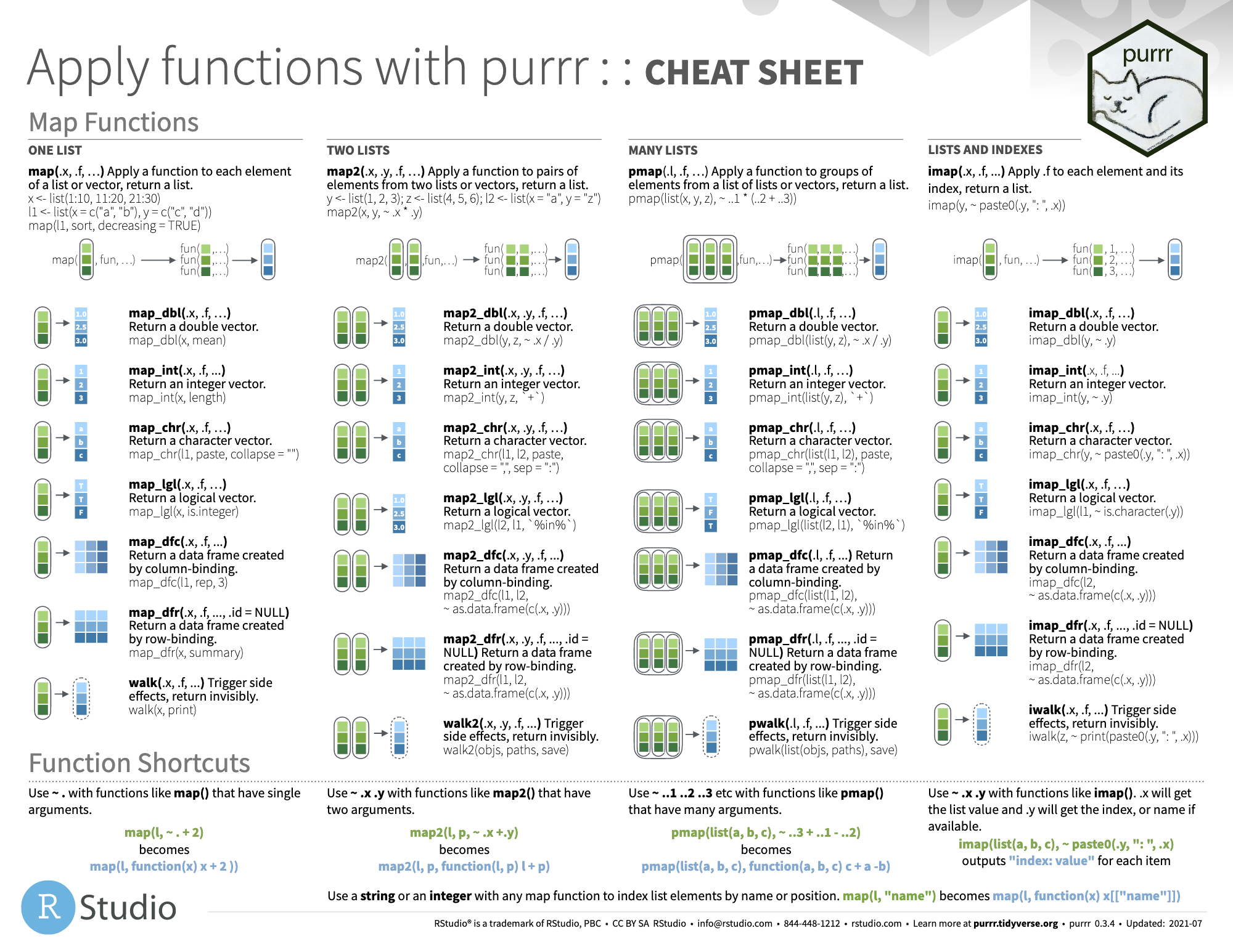
Lists
The simplest function of the {purrr} package is the map() function, which applies a vectorized function to each of the elements of a list. Let’s see a first example applied to vectors
map() allows us to “map” each list and apply the function element by element (if applicable).
Be careful
With vectors we have a default vectorization because R performs element-by-element operations. Note that, by default, the output of map is a list.
Lists
Let’s look at another example. Define in a list two samples from 2 normal distributions, of different sample size and different mean. Compute the mean of each one.
Lists
What if we want to calculate the mean of their squared values?
Lists
In addition to being more readable and efficient, with {purrr} we can decide the output format after the operation
- output as numeric (double) vector with
map_dbl() - output as numeric (int) vector with
map_int() - output as character vector with
map_chr() - output as logical vector with
map_lgl()
Lists
Also, if you pass it a number instead of a function, it will return the ith element of each list.
Lists
We can also use pluck() to access to the i-th element of a list
# A tibble: 87 × 14
name height mass hair_color skin_color eye_color birth_year sex gender
<chr> <int> <dbl> <chr> <chr> <chr> <dbl> <chr> <chr>
1 Luke Sk… 172 77 blond fair blue 19 male mascu…
2 C-3PO 167 75 <NA> gold yellow 112 none mascu…
3 R2-D2 96 32 <NA> white, bl… red 33 none mascu…
4 Darth V… 202 136 none white yellow 41.9 male mascu…
5 Leia Or… 150 49 brown light brown 19 fema… femin…
6 Owen La… 178 120 brown, gr… light blue 52 male mascu…
7 Beru Wh… 165 75 brown light blue 47 fema… femin…
8 R5-D4 97 32 <NA> white, red red NA none mascu…
9 Biggs D… 183 84 black light brown 24 male mascu…
10 Obi-Wan… 182 77 auburn, w… fair blue-gray 57 male mascu…
# ℹ 77 more rows
# ℹ 5 more variables: homeworld <chr>, species <chr>, films <list>,
# vehicles <list>, starships <list>Lists
We also have the option of generalizing it to be able to use functions that need two arguments in the form of a list (binary operations), with map2()
Lists
We can obtain the output in the form of data.frame by adding list_rbind() or list_cbind(), which converts a list into a table.
Lists
We can generalize it further with pmap_xxx() which allows us to use multiple arguments (multiple lists).
Lists
We have other types of iterators that, although they assume inputs, do not return anything, as walk() (just one input argument), walk2() (two arguments) and pwalk() (multiple arguments), all invisibly return, just call a function for its side effects rather than its return value.
💻 It’s your turn
📝 Define a list of 4 elements of different types and access the second of them (I will include one that is a tibble so that you can see that in a list there is room for everything).
📝 From the list above, access the elements that occupy places 1 and 4 of the list defined above.
📝 Load the starwars dataset from the {dplyr} package and access the second movie that appears in starwars$films (for each character). Determine which ones do not appear in more than one movie.
[1] FALSE FALSE FALSE FALSE FALSE FALSE FALSE TRUE TRUE FALSE FALSE FALSE
[13] FALSE FALSE TRUE FALSE FALSE TRUE FALSE FALSE FALSE TRUE TRUE FALSE
[25] TRUE FALSE TRUE TRUE TRUE TRUE TRUE FALSE TRUE FALSE FALSE TRUE
[37] TRUE TRUE FALSE TRUE TRUE FALSE TRUE TRUE FALSE TRUE TRUE TRUE
[49] TRUE FALSE FALSE FALSE FALSE FALSE FALSE TRUE FALSE FALSE TRUE TRUE
[61] TRUE FALSE FALSE TRUE TRUE FALSE FALSE TRUE TRUE TRUE TRUE TRUE
[73] TRUE FALSE TRUE TRUE FALSE TRUE TRUE FALSE FALSE TRUE TRUE TRUE
[85] TRUE TRUE TRUEQuali: factors
In statistics, when we talk about qualitative variables, we will call levels or modalities the different values that these data can take. For example, in the case of the sex variable of the starwars set, we have 4 allowed levels: female, hermaphroditic, male and none (in addition to missing data).
Quali: factors
These kinds of variables are known in R as factors, and the fundamental package to deal with them is {forcats} (from the {tidyverse} environment).
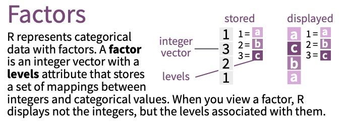
Quali: factors
This package allows us to set the levels (stored internally as levels) that a given categorical variable takes so that no mistakes, errors in data collection and generation can be generated. It also makes their analysis less computationally expensive when doing searches and comparisons, giving them a different treatment than normal text strings.
Let’s see a simple example simulating a party variable taking the values "PP", "PSOE" and "SUMAR" (of size 15)
[1] "PP" "PSOE" "SUMAR" "PP" "PP" "SUMAR" "PSOE" "SUMAR" "SUMAR"
[10] "SUMAR" "PP" "PSOE" "PP" "PSOE" "SUMAR"The party variable is currently of type text, of type chr, something we can check with class(state).
Quali: factors
From a statistical and computational point of view, for R this variable right now would be equivalent to a named variable. But statistically a variable as a string is not the same as a categorical variable that can only take those 3 levels. How to convert to factor?
By making use of the as_factor() function from the {forcats} package.
Quali: factors
Not only the class of the variable has changed, but now, below the saved value, the sentence Levels: ... appears: these are the modalities or levels of our qualitative.
Quali: factors
Imagine that we are defining the database of deputies of the Congress and that the deputies of the PP did not attend that day to the plenary session: although our variable does not take that value THAT DAY, the state PSOE is a allowed level in the database (so even if we eliminate it, because it is a factor, the level remains, we do not have it now but it is an allowed level).
Quali: factors
With factor() function we can explicitly specify the names of the modalities and using levels = ... we can explicitly tell it the “order” of the modalities
Quali: factors
The previous “order” is just in the sense which it will be counted/plotted first) but we don’t have (yet) an ordinal variable
What if we want to define a qualitative variable ORDINAL? Inside factor() we must indicate that ordered = TRUE.
marks <- c("A", "E", "F", "B", "A+", "A", "C", "C", "D", "B", "A", "C", "C", "E", "F", "D", "A+")
marks_database <-
tibble("student" = 1:length(marks),
"marks" =
factor(marks, levels = c("F", "E", "D", "C", "B", "A", "A+"),
ordered = TRUE))
marks_database |> pull(marks) [1] A E F B A+ A C C D B A C C E F D A+
Levels: F < E < D < C < B < A < A+Quali: factors
What changes? If you notice now, although the variable is still qualitative, we can make comparisons and order the records because there is a hierarchy between the modalities.
Quali: factors
If we want to tell it to drop an unused level at that moment (and that we want to exclude from the definition) we can do it with fct_drop().
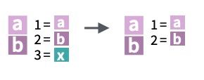
Quali: factors
Just as we can delete levels we can expand existing levels (even if there is no data for that level at that time) with fct_expand().
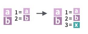
Quali: factors
In addition with fct_explicit_na() we can assign a level to the missing values to be included in the analysis and visualizations.
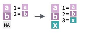
Quali: factors
Even once defined we can reorder the levels with fct_relevel().
Quali: factors
This way of working with qualitative variables allows us to give a theoretical definition of our database, and we can even count values that do not yet exist (but could), making use of fct_count().
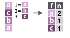
Quali: factors
The levels can also be sorted by frequency with fct_infreq().
[1] A E F B A+ A C C D B A C C E F D A+
Levels: C < A < F < E < D < B < A+# A tibble: 7 × 2
f n
<ord> <int>
1 C 4
2 A 3
3 F 2
4 E 2
5 D 2
6 B 2
7 A+ 2Quali: factors
Sometimes we will want to group levels, for example, not allowing levels that do not happen a minimum number of times with fct_lump_min(..., min = ..) (observations that do not meet this will go to a generic level called Other, although this can be changed with the other_level argument).
Quali: factors
We can do something equivalent but based on its relative frequency with fct_lump_prop().
Quali: factors
We can apply this to our datasets to recategorize variables very quickly.
Quali: factors
With fct_reorder() we can also indicate that we want to order the factors according to a function applied to another variable.
[1] Human Droid Droid Human Human Human Human Droid Human Human
[11] Human Human Others Human Others Others Human Others Human Human
[21] Droid Others Human Human Others Human Others Others Human Others
[31] Human Human Gungan Gungan Gungan Human Others Others Human Human
[41] Others Others Others Others Others Others Others Human Others Others
[51] Others Others Others Others Others Others Human Others Others Others
[61] Human Human Human Human Others Others Others Others Human Droid
[71] Others Others Others Others Others Human Others
Levels: Droid Gungan Human Others [1] Human Droid Droid Human Human Human Human Droid Human Human
[11] Human Human Others Human Others Others Human Others Human Human
[21] Droid Others Human Human Others Human Others Others Human Others
[31] Human Human Gungan Gungan Gungan Human Others Others Human Human
[41] Others Others Others Others Others Others Others Human Others Others
[51] Others Others Others Others Others Others Human Others Others Others
[61] Human Human Human Human Others Others Others Others Human Droid
[71] Others Others Others Others Others Human Others
Levels: Droid Others Human Gungan💻 It’s your turn
📝 Given the variable months defined below (defined as a character vector), convert this variable to factor (just that)
📝 Given the variable months defined below converts this variable to a factor but indicating the levels correctly.
📝 Count how many values there are for each month but keep in mind that they are factors (maybe there are unused levels and you should get a 0 for them).
📝 Since there are missing values, it indicates that the absentee is a thirteenth level labeled "missing".
🐣 Case study I: CIS feminism
We are going to work again with file contains data from the CIS (Centro de Investigaciones Sociológicas) barometer «Perceptions on equality between men and women and gender stereotypes» whose sample work was carried out from November 6 to 14 (4000 interviews of both sexes over 16 years old in 1174 municipalities and 50 provinces).
Try to answer the questions posed in the workbook
L9: dbplyr and github
dbplyr: SQL connection
We are going to introduce the {dbplyr} package, which will allow us to combine SQL code into R to perform database queries
If you are using R to do data analysis, most of the data you need probably already lives in a database. We will learn how to load data in to a local database.
dbplyr: SQL connection
We will also need to install a DBI backend package (an interface that allows {dplyr} to work with many different databases using the same code). Five commonly used backends are:
RMariaDBconnects to MySQL and MariaDBRPostgresconnects to Postgres and Redshift.RSQLiteembeds a SQLite database.odbcconnects to many commercial databases via the open database connectivity protocol.bigrqueryconnects to Google’s BigQuery.
In the following, we are going to use the RSQLite backend (automatically installed when you install {dbplyr}).
dbplyr: SQL connection
If we want to work with a database adopting dplyr grammar, we must first connect to it. The connection will be done by using DBI::dbConnect(). The arguments to DBI::dbConnect() vary from database to database, but the first argument is always the database backend. SQLite only needs a path to the database.
<SQLiteConnection>
Path: :memory:
Extensions: TRUEHere, the string ":memory:" is a special path that creates a temporary in-memory database.
dbplyr: SQL connection
The temporary database previously created has no yet data in it. We will copy an existing database (for example, gapminder from {gapminder} package) using copy_to(). Using tbl() we “obtain” the database (called as named in copy_to()).
The main difference is that not it is a remote source in a SQLite database.
copy_to(connection, gapminder::gapminder, overwrite = TRUE, name = "gapminder_database")
gapminder_db <- tbl(connection, "gapminder_database")
gapminder_db# Source: table<`gapminder_database`> [?? x 6]
# Database: sqlite 3.43.2 [:memory:]
country continent year lifeExp pop gdpPercap
<chr> <chr> <int> <dbl> <int> <dbl>
1 Afghanistan Asia 1952 28.8 8425333 779.
2 Afghanistan Asia 1957 30.3 9240934 821.
3 Afghanistan Asia 1962 32.0 10267083 853.
4 Afghanistan Asia 1967 34.0 11537966 836.
5 Afghanistan Asia 1972 36.1 13079460 740.
6 Afghanistan Asia 1977 38.4 14880372 786.
7 Afghanistan Asia 1982 39.9 12881816 978.
8 Afghanistan Asia 1987 40.8 13867957 852.
9 Afghanistan Asia 1992 41.7 16317921 649.
10 Afghanistan Asia 1997 41.8 22227415 635.
# ℹ more rowsdbplyr: SQL connection
The main goal of {dbplyr} is to automatically generate SQL from dplyr grammar that we are already familiar with.
# Source: SQL [?? x 3]
# Database: sqlite 3.43.2 [:memory:]
country year lifeExp
<chr> <int> <dbl>
1 Afghanistan 1952 28.8
2 Afghanistan 1957 30.3
3 Afghanistan 1962 32.0
4 Afghanistan 1967 34.0
5 Afghanistan 1972 36.1
6 Afghanistan 1977 38.4
7 Afghanistan 1982 39.9
8 Afghanistan 1987 40.8
9 Afghanistan 1992 41.7
10 Afghanistan 1997 41.8
# ℹ more rowsdbplyr: SQL connection
The most important difference between ordinary tibbles and remote database queries is that now our R code is translated into SQL and executed in the database on the remote server, not in R on your local machine: it never pulls data into R unless you explicitly ask for it, delaying doing any work until the last possible moment (sends it to the database in one step).
It is not until we ask for the data (writing gapminder_query in console, for example), dplyr verbs generates the SQL and requests the results from the database.
# Source: SQL [?? x 3]
# Database: sqlite 3.43.2 [:memory:]
country year lifeExp
<chr> <int> <dbl>
1 Afghanistan 1952 28.8
2 Afghanistan 1957 30.3
3 Afghanistan 1962 32.0
4 Afghanistan 1967 34.0
5 Afghanistan 1972 36.1
6 Afghanistan 1977 38.4
7 Afghanistan 1982 39.9
8 Afghanistan 1987 40.8
9 Afghanistan 1992 41.7
10 Afghanistan 1997 41.8
# ℹ more rowsdbplyr: SQL connection
What is happening behind the scenes?
dbplyr: SQL connection
As commented, our remote database queries is not in R on your local machine: it never pulls data into R unless you explicitly ask for it. To do it, you can iterate a few times before you figure out what data you need, and then we use collect().
# A tibble: 1,704 × 3
country year lifeExp
<chr> <int> <dbl>
1 Afghanistan 1952 28.8
2 Afghanistan 1957 30.3
3 Afghanistan 1962 32.0
4 Afghanistan 1967 34.0
5 Afghanistan 1972 36.1
6 Afghanistan 1977 38.4
7 Afghanistan 1982 39.9
8 Afghanistan 1987 40.8
9 Afghanistan 1992 41.7
10 Afghanistan 1997 41.8
# ℹ 1,694 more rowsdbplyr: SQL connection
You can also use translate_sql() to translate individual expressions from dplyr to SQL
What about Github?
GitHub is the most well-known collaborative platform based on the Git version control system
- What is Git? Git is a version control system: a kind of Dropbox to facilitate collaborative programming among a group of people, allowing to keep track of the traceability of changes made.
- What is Github? Our platform/interface for running version control: it will serve us not only to work collaboratively but to make transparent the process of building our code projects.
Important
As of June 4, 2018 Github is owned by Microsoft (ergo the code you upload as well).
Overview
After making an account in Github, up right we will have a circle, and clicking on Your Profile, we will see something like this

Edit profile: allows us to add a description and profile picture.
Overview: in that squares panel will view our activity over time.
Repositories: the code will be uploaded to repositories, the equivalent of our shared folders in Dropbox.
First use
Before learning how to create repositories, Github will also be useful to
Access code from others
Propose improvements to other users, and even propose bug fixes we detect for software we use.
- Install R packages]{.hl-purple}. In many cases package developers upload updates to CRAN from time to time, and in other cases the software is not “wide” enough to be uploaded as a package.
Package code that is not uploaded to CRAN can be installed as code from Github
Installing from Github
For example, let’s install a package called {peRReo}, whose only function is to give us color palettes based on urban music albums covers.

Installing from Github
The installation instructions are usually detailed in the repository cover page (README.md file)

Installing from Github
Most of the time what we upload will not be an R package as such but we will upload a more or less organized and commented code. In that case we can download the whole repo by clicking Code and then Download ZIP.
For example, let’s download the dataviz scripts that have been uploaded from the Centre d’Estudis d’Opinió (Catalan CIS).
First repo
Let’s create our first repository that will also serve as the cover page of our Github profile.
Repositories: click on the Repositories tab.
New: click on the New button to create a new repository.
First repo
Repository name: the repository name. In this case we are going to create a very specific repository: the name must exactly match your username
Description: description of your repository. In this case it will be a presentation repo.
![]()
First repo
Public vs private: with each repository we will have the option to make the repository
- public: all users will be able to see the code as well as the traceability of your development (what is added and when). It is for me the most recommended option when you want to give visibility and transparency to your work
- private: only those users you allow will have access to the repository. Nothing can be viewed or installed from it outside of Github.

In this particular case, since it will be a presentation repository, we will make it public.
First repo
- Add a README file]{.hl-purple}: a README file will be the file where we will include the instructions and usage details to the others (in the case of
{peRReo}it was the file containing the installation details).
For the time being ignore other fields for this first repository.
First repo
By default Github assumes that this repository, with the same name as our user will be the repository we want to be presented at startup when someone logs into our profile, and will be the repository where include in the README.md a presentation of us and an index of your work (if you want).
First repo
Notice that now in our cover page we have said README.md that we can customize to our liking using html and markdown.Here you can see some examples of README.md
Code repo
Once we have our presentation README (remember you can customize to your liking with html and markdown) let’s create a code repository.
If it was already important to work with projects in RStudio, when combined with Github it is even more crucial that we create a project before uploading code, so let’s create a test one called repo-github-1.
In this project we are going to create a script (in my case called codigo.R) in which you must do the following steps:
Code repo
- Download directly from the ISCIII page the file named
casos_hosp_hosp_uci_def_def_sexo_edad_provres.csv.
- Filter data for Madrid (
“M”), between March 1, 2020 and December 31, 2020, and with sex“H”. After that keep the columnsfecha,grupo_edad,num_casos(that order). Finally get the sum of daily cases per date (regardless of age group).
Code repo
- Export the dataset to a csv in a folder named
exported.
Code repo
How do we upload the project? Let’s go back to create a project from scratch. We didn’t talk about two important fields earlier:
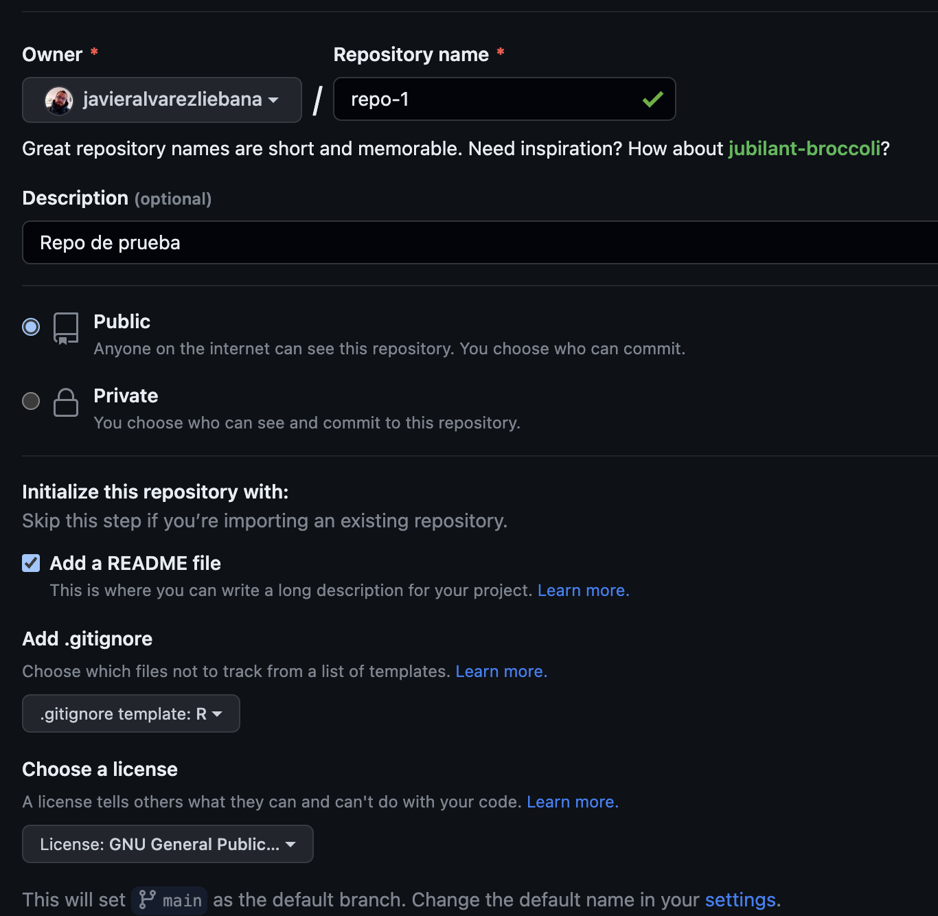
Add .gitignore` will allow us to select the language our project will be in so that Github understands it when syncing (and doesn’t update things it shouldn’t).
Choose a licensewill allow us to select the license which will determine the conditions under which others will be able to reuse your code.
Code repo
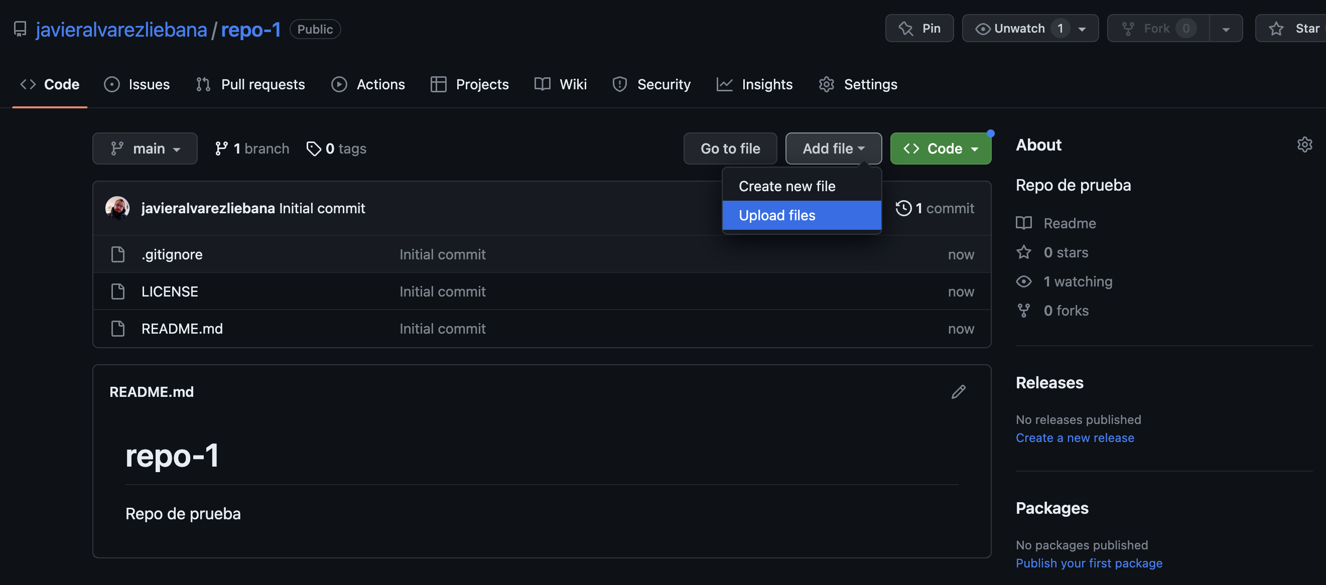
If you look at how to create it we have only 3 files: the license file, the .gitignore and the readme.md (where we should write a user guide of what we have uploaded).
To upload the files we will click on Add file < Upload File and drag ALL files from our project folder.
Code repo
After uploading files we will have a box called Commit changes
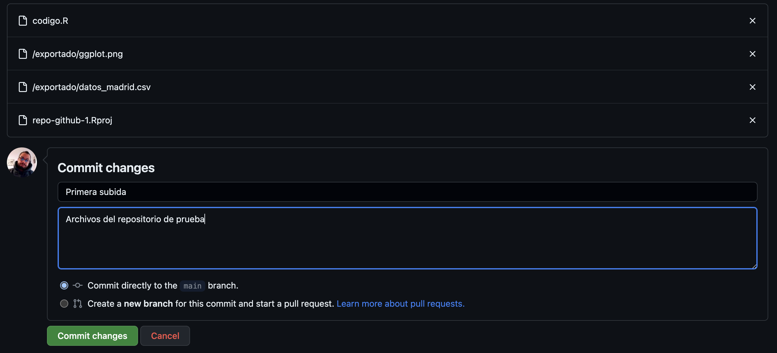
A commit is a modification of the repository with something to be added/removed/modified, and it is advisable to use this box to summarize what the modification is about, so that the change is traced.
Code repo
By clicking on the clock where it indicates the number of commits we access the history of commits (changes) with time, day, author, comments, etc.
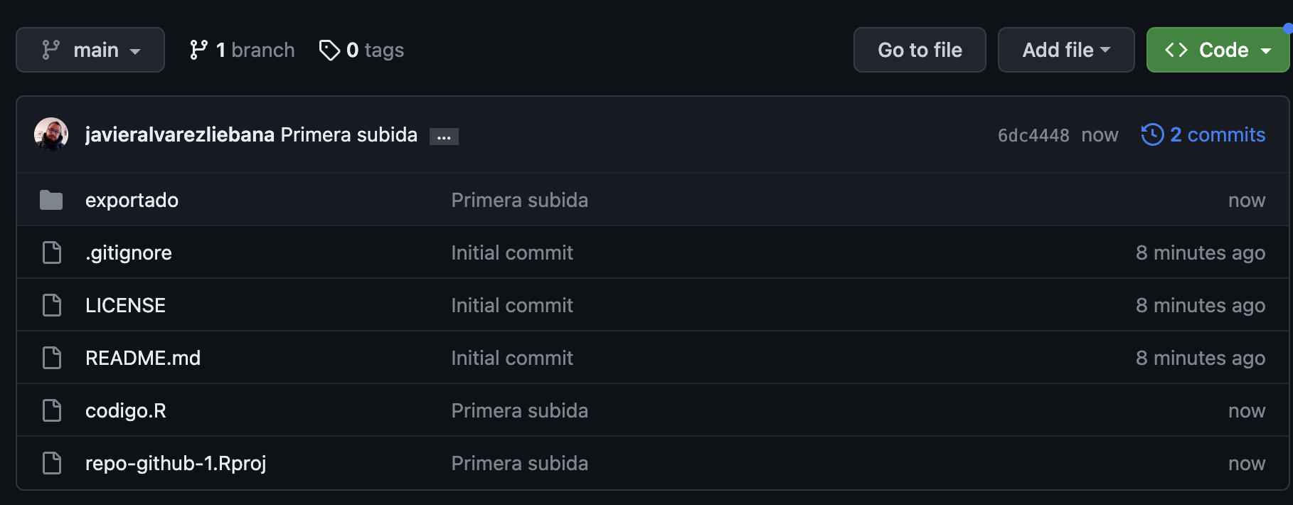
Code repo
Let’s make a change in our code: in your local code (local –> your computer), instead of filtering by Madrid do the filter by Barcelona, save the code and upload the new file in the repository (with the same name, Github will do the overwrite)
Commits
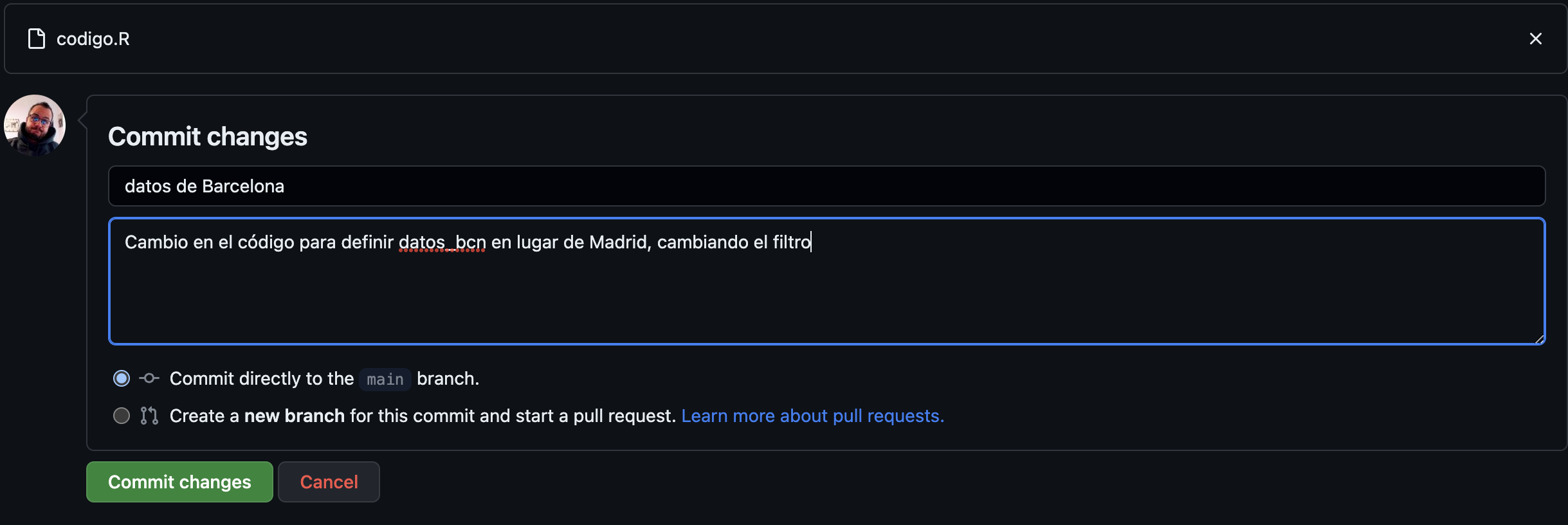
If we now consult the commit, next to it there is a number that identifies it, and clicking on it summarizes the changes: not only stores all past versions but also shows the differences between the changed files

Change traceability


We have two display modes of the changes: the split mode shows us the old and the new, with the inclusions in green and what is no longer there in red; and the unified mode shows us everything in the same document.
Retrieval of commits
Github even allows us to retrieve a past version from our repository by clicking on the third commit icon.
Retrieval of commits
If you notice now next to 1 branch we have a drop-down menu where before it used to say main and now a commit identifier number. We will talk about the idea of branch (branch) later.
Repo with rmd/qmd
Let’s put what we have learned into practice:
Create a new repository in Github (called
repo-github-2) where you will have hosted your R project.Create a project in
RStudiocalled (for example)project-qmdOnce inside the project in
RStudioclick onFile < New File < Quarto Document.
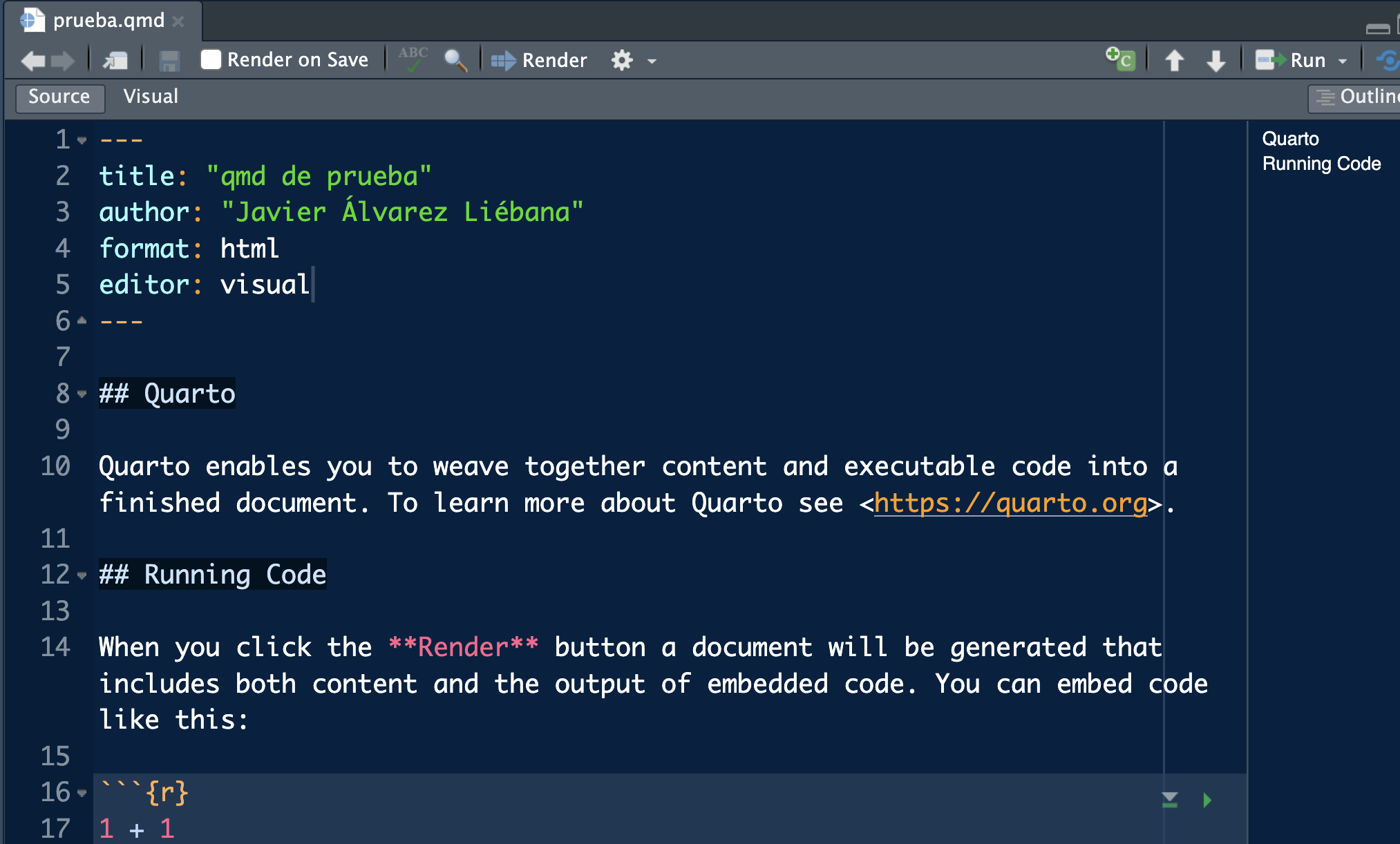
You should have a document similar to this: a fourth markdown (.qmd), a document that will allow us to include markdown + code (it can be R or it can be Observable, D3, etc).
Repo with rmd/qmd
This format is ideal for:
Working in a team building a draft of a piece.
Taking notes or reports for yourself.
Presenting your work to your peers.
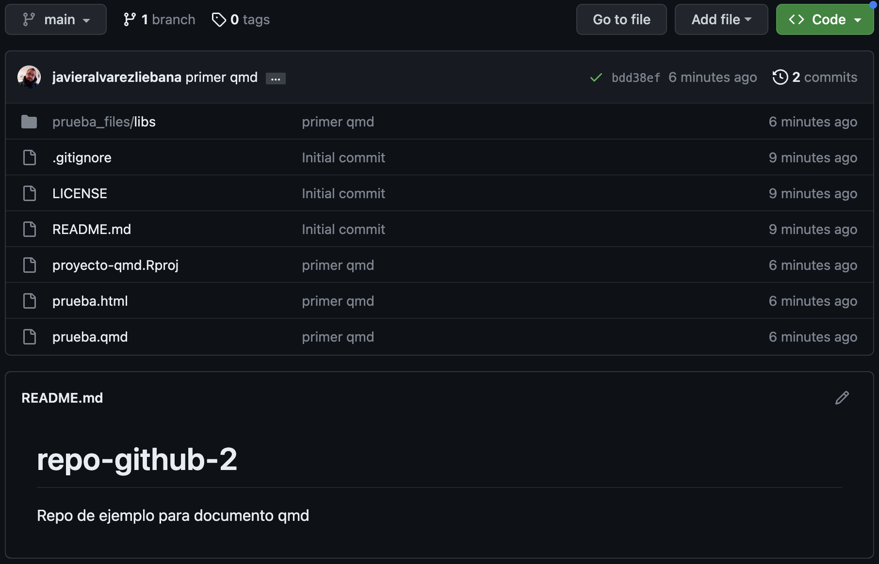
If you notice now our repository has a file with .html format…that is to say….
It’s a web!
Github pages
How to convert our repository properly into a web?
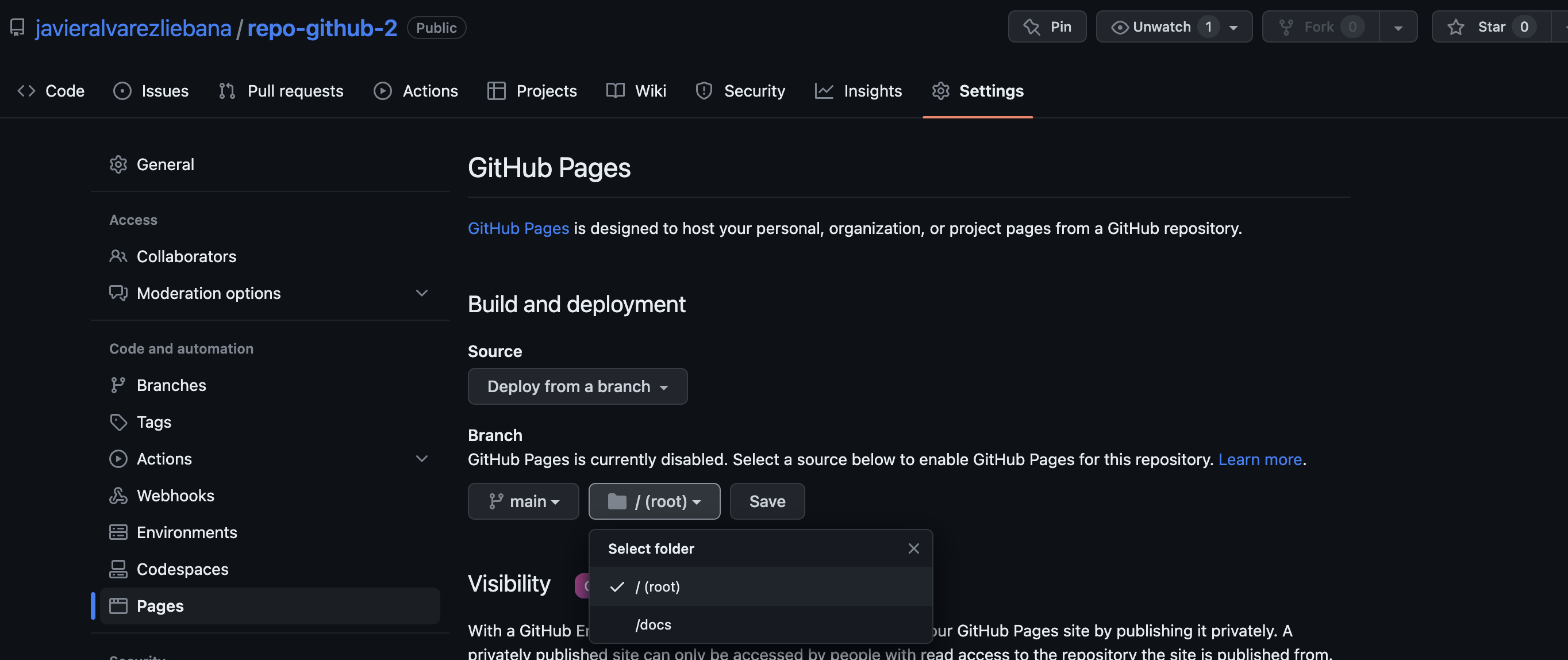
Click on
SettingsGo to
PagesIn the subsection
branchselect the only branch that we have now (main)Select the folder where you have the
.html(in complex web it will be as in any web indocs, in something simple it will be in the root path of the repository)Click on
Save.
Github pages
If you look at the top of the repository now we have an orange icon, which indicates that the web is in the process of being deployed
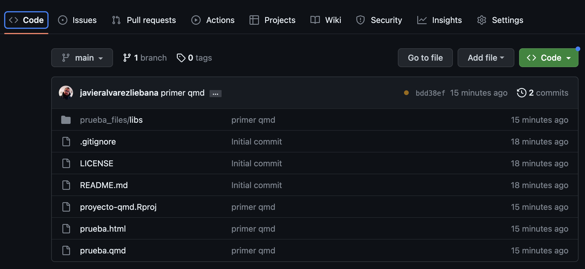
Github pages
After a few seconds (depending on the size of the website and your internet connection) that icon will change to a green check
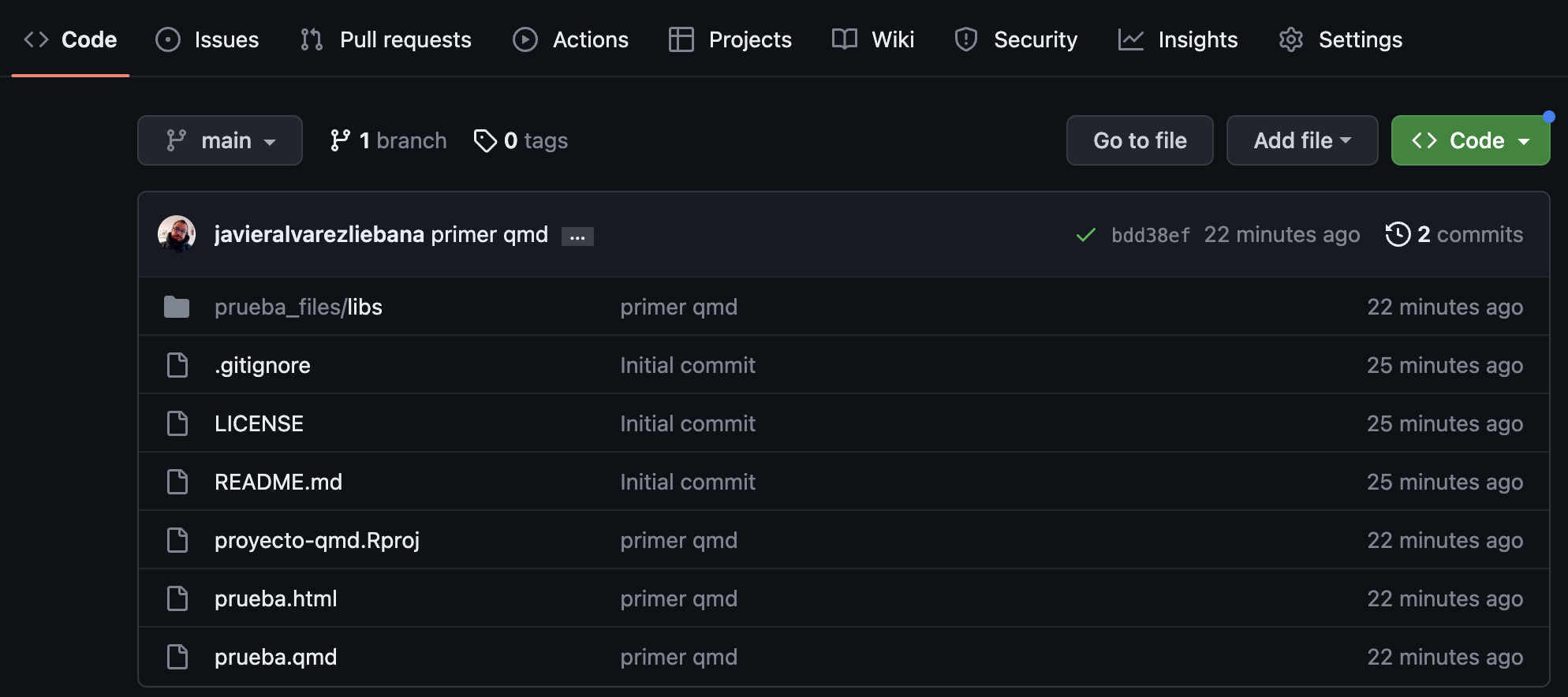
The default web link will be {username}.github.io/{repo_name}.
Github pages
Wait a minute! Right now our website is not showing us our .qmd, but by default the README.md.
For Github to understand that we want to display that .html that we have generated from the .qmd we go in our local project to delete everything that is not our .Rproj file and our .qmd file, and we go to name the latter calling it index.qmd, and we recompile it to generate an index.html
Github pages
Let’s upload to Github that new project with the name change (called repo-github-3) to see later the differences between one and the other one.
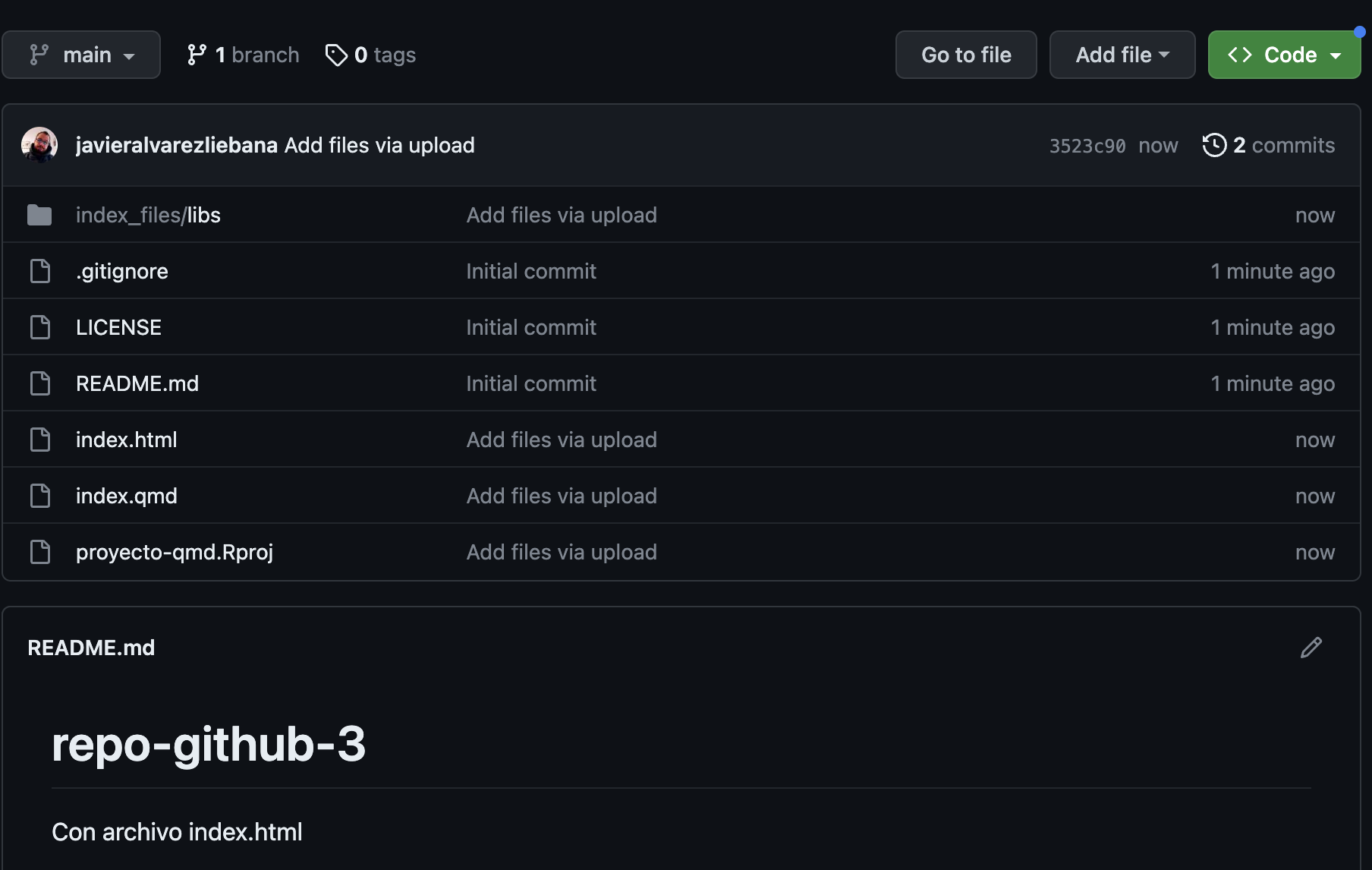
Github pages
If we repeat the process to make a Page and wait for the green tick…
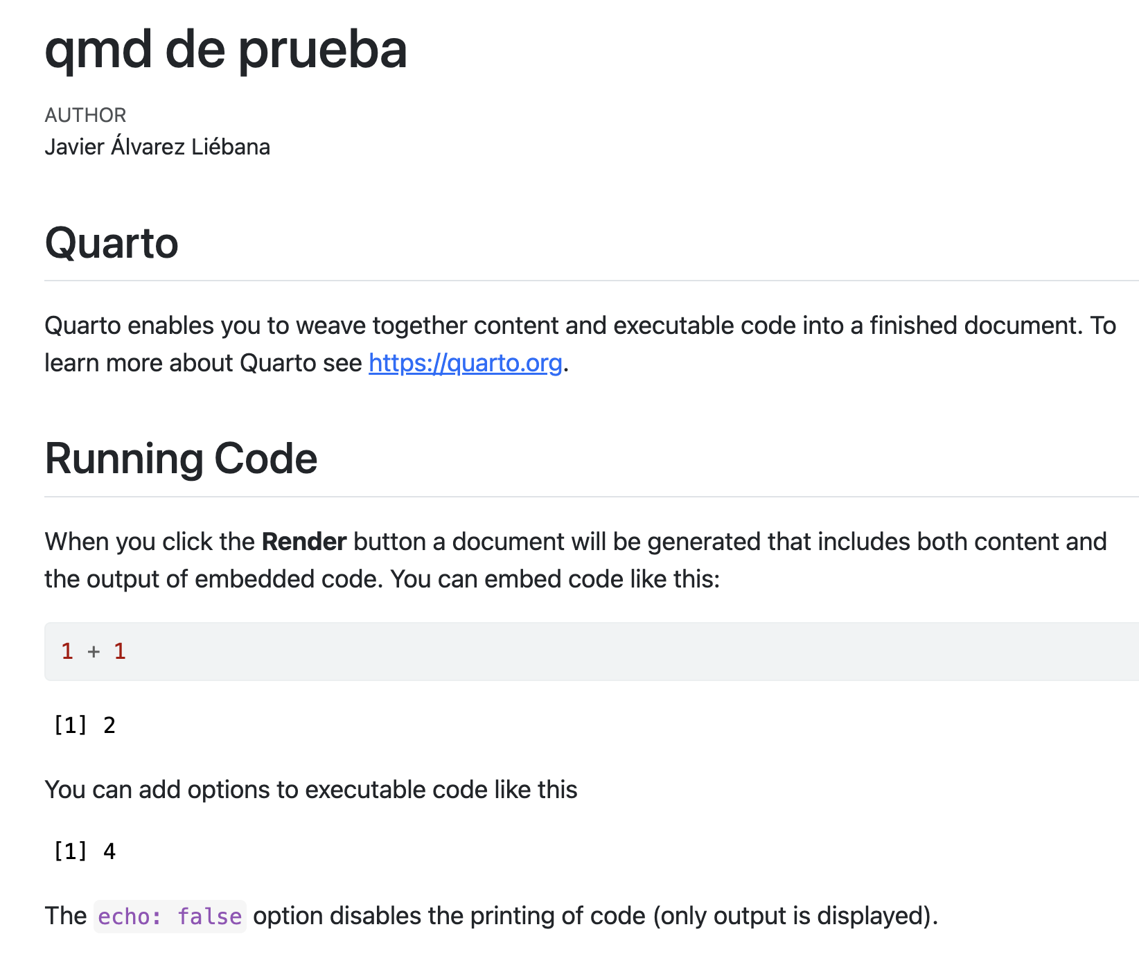
If your .qmd is already called index.qmd, automatically, when Github detects an index.html, it interprets that index.html file is the one that defines the web (and you can customize by adding a css style file)
We have a web by simply clicking on Pages :)
Repo with slides
Let’s create the last repository which will be called repo-diapos, and create a project in RStudio of the same name (for example). Once created we will click on File < New File < Quarto Presentation.
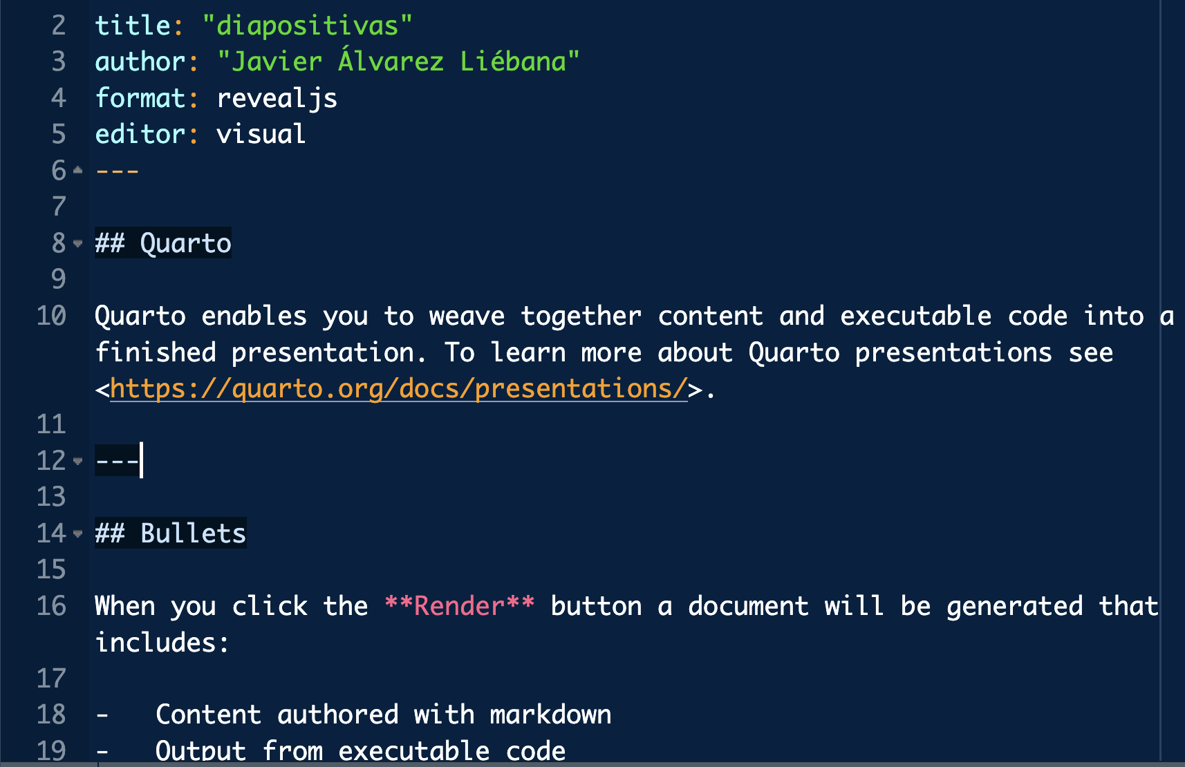
The way to write will be the same as a normal .qmd only now each slide will be separated with a --- (using style files we can customize whatever we want)
Call the file directly index.qmd, upload it to Github and with one click in Pages you have a web with your slides
Github Desktop
pending
Javier Álvarez Liébana • Master in Computational Social Sciences (UC3M)

